1. The Core Engineering Challenge: The Accelerator Memory Wall
Training frontier Artificial Intelligence models with tens or hundreds of billions of parameters (such as Llama 3 70B, GPT-4, or Gemini) is fundamentally constrained by a single physical bottleneck: High-Bandwidth Memory (HBM) capacity on accelerator chips.
Consider the hardware reality of a modern data-center accelerator, the NVIDIA H100 SXM5 (80 GB):
- Compute Throughput: dense FP16/BF16 Tensor Cores ( with 2:4 structured sparsity; dense FP8 / sparse FP8). Compare with NVIDIA A100 SXM4 (80 GB) at dense BF16 ( sparse).
- HBM Capacity: HBM3 on H100 SXM5 ( HBM3e on H200 SXM, HBM3e on Blackwell B200).
- Memory Bandwidth & Roofline Ridge Point: on H100 SXM5, yielding a dense BF16 Roofline ridge point of (versus on A100 SXM4).
Now calculate the memory required to train a 70-Billion Parameter () dense Transformer model (using decimal , and noting binary in parentheses):
If we load this model in 16-bit floating-point format (FP16 or BF16, where each parameter occupies ), the static model weights alone consume:
already exceeds the entire physical HBM3 capacity of a single H100! And this accounts only for the weights. As we will prove, mixed-precision Adam training requires more static memory than 16-bit inference: full mixed-precision training demands per parameter (, or for ), completely exceeding single-chip capacity.
To train modern models within weeks rather than centuries, we must distribute computation, gradients, activations, and optimizer states across thousands of GPUs coordinated by ultra-high-speed network fabrics.
2. Mental Model: 3D Parallelism & The Interconnect Hierarchy
Distributed training is governed by a strict physical hierarchy of interconnect bandwidths:
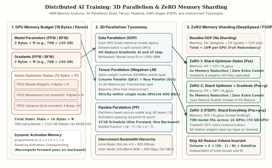
1. Model Parameters (FP16 / BF16) & Gradients (FP16 / BF16)
Establishes the ingress and structural boundary across Model Parameters (FP16 / BF16) & Gradients (FP16 / BF16): 2 Bytes × Ψ (e.g., 70B = 140 GB).
2. Adam Optimizer States (12 Bytes × Ψ) & FP32 Master Weights: 4 Bytes × Ψ
Coordinates core data-plane execution and state transitions through Adam Optimizer States (12 Bytes × Ψ) & FP32 Master Weights: 4 Bytes × Ψ: proportional to: b × s × h × L × a; Saved by Activation Checkpointing (Recompute forward pass on backward); Each GPU holds identical model replica Dataset batch is split across GPUs All-Reduce Gradients at end of step.
3. Baseline DDP (No Sharding) & ZeRO-1: Shard Optimizer States (Pos)
Enforces durability, state convergence, and output verification across Baseline DDP (No Sharding) & ZeRO-1: Shard Optimizer States (Pos): Memory: 2Ψ (weights) + 2Ψ (grads) + 12Ψ (opt); Total = 16Ψ per GPU (Full Redundancy); Memory: 4Ψ + 12Ψ / N_gpus.
+-------------------------------------------------------------------------------+
|                       THE ACCELERATOR INTERCONNECT HIERARCHY                  |
+-------------------------------------------------------------------------------+
| Domain           | Technology            | Unidirectional Bandwidth| Latency  |
+------------------+-----------------------+-------------------------+----------+
| 1. On-Chip       | HBM3 / HBM3e Memory   | 3,350 GB/sec (3.35 TB/s)| ~50 ns   |
| 2. Intra-Node    | NVLink 4.0 (8 GPUs)   | 450 GB/sec (900 GB/s bi)| ~500 ns  |
| 3. Inter-Node    | InfiniBand Quantum-2  | 50 GB/sec (400 Gbps NDR)| ~2-5 µs  |
| 4. Data Center   | RoCEv2 (Ethernet)     | 12.5 - 25 GB/sec        | ~10-25 µs|
+-------------------------------------------------------------------------------+
Because intra-node NVLink is 18x faster than inter-node InfiniBand, distributed training pipelines decompose model architectures using 3D Parallelism:
- Tensor Parallelism (TP): Splits individual weight matrices across GPUs within the same physical node (e.g. 8 GPUs connected via NVLink).
- Pipeline Parallelism (PP): Partitions sequential Transformer layers across different server nodes (connected via InfiniBand), using point-to-point activation passing.
- Data Parallelism (DP / DDP): Replicates the model across multiple nodes, sharding the dataset batches across the cluster and synchronizing gradients via collective All-Reduce operations.
Foundational Bridge: Transformer Compute/Memory Anatomy, Roofline Intensity & Mixed-Precision Formats
Before partitioning a frontier LLM across thousands of GPUs via 3D parallelism, we must derive the exact byte and FLOP budgets of a single Transformer decoder layer:
- Parameter & FLOP Scaling Laws (Per Token, Per Layer):
- For hidden dimension , intermediate MLP dimension (or in SwiGLU), and layers, total parameter count scales as .
- A forward pass executes one multiply-accumulate () per parameter per token (). The backward pass computes gradients with respect to both activations and weights (), yielding per training step ( total FLOPs over dataset size tokens).
- Why Training Memory Exceeds Inference Memory by :
- Inference requires storing only model weights (e.g., in
BF16) plus the dynamic KV cache for active sequences; intermediate layer activations are discarded immediately after each layer completes. - Training must retain every intermediate forward-pass activation tensor across all layers in HBM until the backward pass traverses back through that layer to compute , alongside Weights (), Gradients (), and FP32 Adam Optimizer States (: master weights, first moment , second moment )—totalling of static model state before activations!
- Activation Checkpointing (Recomputation): Discards intermediate layer activations during the forward pass (keeping only layer boundary inputs) and recomputes them on-the-fly during backpropagation, trading extra compute FLOPs for an reduction in activation HBM footprint.
- Inference requires storing only model weights (e.g., in
- Numeric Precision Formats (
FP32vs.FP16vs.BF16vs.FP8):FP32(1 sign, 8 exponent, 23 mantissa bits): High precision, but slow tensor-core throughput and .FP16(1 sign, 5 exponent, 10 mantissa bits): Narrow dynamic range (); small gradients underflow to zero, requiring Dynamic Loss Scaling.BF16(Brain Float 16: 1 sign, 8 exponent, 7 mantissa bits): MatchesFP32’s exact 8-bit exponent dynamic range (), eliminating gradient underflow without loss scaling during LLM pre-training.FP8(E4M3for forward activations/weights with higher precision;E5M2for backward gradients needing wider range): Doubles Hopper/Blackwell Tensor Core throughput ( TFLOPS overBF16) with per-tensor or blockwise scaling factors.
3. Mathematical Model: GPU HBM Memory Accounting
During training, memory is split into two categories: Static Model States (which scale strictly with parameter count ) and Dynamic Residual States (which scale with batch size and sequence length).
1. Static Model States: The Rule
To train with stability, deep neural networks use Mixed-Precision Training (Micikevicius et al., 2018):
+-------------------------------------------------------------------------------+
|                   MIXED-PRECISION ADAM MEMORY ALLOCATION                      |
+-------------------------------------------------------------------------------+
| Component           | Precision | Bytes per Param | Formula for Ψ = 70B       |
+---------------------+-----------+-----------------+---------------------------+
| 1. Model Weights    | FP16/BF16 | 2 bytes         | 140 GB                    |
| 2. Gradients        | FP16/BF16 | 2 bytes         | 140 GB                    |
| 3. Master Weights   | FP32      | 4 bytes         | 280 GB                    |
| 4. Adam Momentum    | FP32      | 4 bytes         | 280 GB                    |
| 5. Adam Variance    | FP32      | 4 bytes         | 280 GB                    |
+---------------------+-----------+-----------------+---------------------------+
| TOTAL STATIC MEMORY | Mixed     | 16 bytes / param| 1,120 GB (1.12 TB!)       |
+---------------------+-----------+-----------------+---------------------------+Why 12 Bytes for Adam States?
During backward propagation, gradient updates are often on the order of or . In standard 16-bit floating point (FP16), numbers smaller than suffer catastrophic numerical underflow to zero! To prevent weights from stalling, the Adam optimizer maintains an authoritative FP32 Master Copy of the weights, along with two running statistics: the FP32 First Moment (Momentum) and the FP32 Second Moment (Variance). This requires of optimizer state per parameter.
2. Dynamic Activation Memory
Activations are the intermediate tensor outputs saved during the forward pass so they can be reused to compute gradients during the backward pass.
For a standard mixed-precision Transformer without Tensor Parallelism or FlashAttention, with sequence length , hidden dimension , number of attention heads , micro-batch size , and number of layers (Korthikanti et al., 2022):
(Note: When using FlashAttention-2/3, the full attention score matrix is never materialized in HBM, eliminating the quadratic term so total activation memory scales linearly as bytes, further divided by under -way Tensor + Sequence Parallelism.)
For long context windows (e.g. or tokens), activation memory quickly explodes to tens of gigabytes per GPU, frequently exceeding static model memory!
Activation Checkpointing (Gradient Checkpointing)
Rather than storing all intermediate layer activations in HBM:
- The engine stores only the input tensor to each Transformer block ().
- During the backward pass, the forward pass for that specific block is recomputed on-the-fly.
- Trade-off: Recomputation costs additional FLOPS, but slashes activation memory by up to , making long-context training possible.
4. Data Parallelism (DDP) & The Ring All-Reduce Primitive
In standard Distributed Data Parallel (DDP):
- Every GPU holds an identical copy of all model parameters and optimizer states.
- The global training batch (e.g., sequences) is split into micro-batches distributed across GPUs (e.g., sequences per GPU across GPUs).
- Each GPU computes its local forward and backward pass, generating local gradients .
- Before updating optimizer states, all GPUs must compute the average gradient across the entire cluster:
The Ring All-Reduce Algorithm
A naive approach where all GPUs send their gradients to a central parameter server causes an immediate network interface bottleneck at the master node.
In 2017, Baidu Research adapted the Ring All-Reduce algorithm for deep learning, maximizing interconnect bandwidth across ring topologies (such as NVIDIA NCCL):
Ring All-Reduce Topology (N = 4 GPUs):
---------------------------------------------------------------------------------
Each GPU arranges its gradient buffer of size M into N equal chunks:
Chunk 0, Chunk 1, Chunk 2, Chunk 3 (each chunk size = M / N)

      +----------> [ GPU 0 ] ---------->+
      |                                 |
      |                                 v
   [ GPU 3 ]                         [ GPU 1 ]
      ^                                 |
      |                                 |
      +----------< [ GPU 2 ] <----------+

Phase 1: Reduce-Scatter (N - 1 = 3 steps)
Step 1: GPU i sends Chunk i to GPU (i + 1), and receives Chunk (i - 1) from GPU (i - 1).
        GPU sums received chunk with its local chunk.
Step 2: GPU i sends the accumulated chunk forward.
...
Result of Phase 1: Each GPU holds the fully summed global value for exactly ONE chunk!

Phase 2: All-Gather (N - 1 = 3 steps)
Each GPU sends its fully summed chunk around the ring until all nodes possess all chunks.
Derivation: Ring All-Reduce Communication Invariant
Let be the total gradient buffer size in bytes, and be the number of GPUs in the ring:
- In the Reduce-Scatter phase, each GPU sends bytes in each of the steps:
- In the All-Gather phase, each GPU again sends bytes across steps:
Total data transferred per GPU during the entire All-Reduce operation is:
As the cluster size grows large ():
Crucial Insight: The communication volume per GPU is completely independent of the cluster size ! Whether training across 8 GPUs or 4,096 GPUs, each GPU transmits almost exactly bytes of gradient data per step.
5. Tensor Parallelism: Megatron-LM Matrix Decomposition
When an individual Transformer layer cannot fit in single GPU memory, we must shard the weight matrices inside the self-attention and multi-layer perceptron (MLP) blocks.
Introduced by Shoeybi et al. (Megatron-LM, 2019), Tensor Parallelism (TP) splits matrix multiplications (GEMM) across GPUs while minimizing synchronization points.
1. Multi-Head Attention Sharding
In self-attention, input tensor is projected into Query (), Key (), and Value () matrices, followed by an output projection :
Megatron-LM Attention Matrix Sharding:
---------------------------------------------------------------------------------
1. Column-Parallel Projection:
   Split Q, K, V projection matrices vertically across N GPUs:
   GPU 0: W_Q1, W_K1, W_V1  --> Computes local Q1, K1, V1
   GPU 1: W_Q2, W_K2, W_V2  --> Computes local Q2, K2, V2
   --> ZERO COMMUNICATION NEEDED! (Each GPU computes local attention heads)

2. Row-Parallel Projection:
   Split Output matrix W_O horizontally:
   GPU 0: W_O1 (multiplied with local Attention_1)
   GPU 1: W_O2 (multiplied with local Attention_2)

3. All-Reduce Synchronization:
   Output = (Attention_1 · W_O1) + (Attention_2 · W_O2)
   --> Exactly ONE All-Reduce operation in the forward pass!
2. Multi-Layer Perceptron (MLP) Sharding
The MLP block consists of two GEMMs: :
- is sharded Column-Parallel (no communication after GELU activation).
- is sharded Row-Parallel.
- Exactly one All-Reduce at the end of the MLP block sums the partial products.
Why Tensor Parallelism Does Not Scale Across Nodes
Tensor Parallelism requires 2 All-Reduce operations per Transformer layer on every forward pass, and 2 All-Reduces on every backward pass:
If executed over InfiniBand (), network serialization latency stalls the Tensor Cores, dropping GPU compute utilization (MFU) below . Therefore:
6. Pipeline Parallelism: Layer Partitioning & The 1F1B Schedule
To distribute an 80-layer model across nodes, Pipeline Parallelism (PP) assigns subsets of consecutive layers to different GPUs:
- GPU 0: Layers
- GPU 1: Layers
- GPU 2: Layers
- GPU 7: Layers
The Pipeline Bubble Problem
If GPU 0 processes the entire training batch before sending activations to GPU 1, all downstream GPUs sit completely idle waiting for input. This wasted idle time is the Pipeline Bubble.
Naive Pipeline Schedule (Massive Bubble):
---------------------------------------------------------------------------------
GPU 3:                                         [F] [B]
GPU 2:                                 [F]                 [B]
GPU 1:                         [F]                                 [B]
GPU 0:                 [F]                                                 [B]
       Time ---------> |============== IDLE BUBBLE ========================|
The 1F1B (One-Forward-One-Backward) Schedule
To minimize the bubble, the global batch is sliced into micro-batches (Narayanan et al., PipeDream):
- After a short warmup phase, each GPU alternates between executing one forward pass on a new micro-batch and one backward pass on an older micro-batch.
1F1B Steady-State Execution Schedule:
---------------------------------------------------------------------------------
GPU 3:             [F1] [F2] [F3] [F4] [B1] [F5] [B2] [F6] [B3] [B4] [B5] [B6]
GPU 2:        [F1] [F2] [F3] [F4] [B1] [F5] [B2] [F6] [B3] [B4] [B5] [B6]
GPU 1:   [F1] [F2] [F3] [F4] [B1] [F5] [B2] [F6] [B3] [B4] [B5] [B6]
GPU 0: [F1] [F2] [F3] [F4] [B1] [F5] [B2] [F6] [B3] [B4] [B5] [B6]
Pipeline Bubble Fraction Formula
Let be the pipeline depth (number of pipeline stages), and be the number of micro-batches:
To keep the bubble overhead below (), the number of micro-batches must be at least 9 times the pipeline depth:
7. The ZeRO Memory Sharding Revolution (DeepSpeed & PyTorch FSDP)
In 2020, Rajbhandari et al. (Microsoft Research) published ZeRO (Zero Redundancy Optimizer), revealing that standard Data Parallelism wastes colossal amounts of HBM by replicating identical optimizer states and gradients across every single GPU in the cluster.
ZeRO eliminates memory redundancy across data-parallel degree in three progressive stages (shown below for parameters and GPUs in decimal GB):
+-------------------------------------------------------------------------------+
|                      ZeRO / FSDP STAGES MEMORY BREAKDOWN                      |
+-------------------------------------------------------------------------------+
| Sharding Stage      | What is Sharded?         | Memory per GPU (Ψ=70B, Nd=64)|
+---------------------+--------------------------+------------------------------+
| Baseline DDP        | None (Full Redundancy)   | 16Ψ = 1,120.0 GB (OOM!)      |
|                     |                          |                              |
| ZeRO-Stage 1 (Pos)  | Adam Optimizer States    | 4Ψ + 12Ψ/Nd = 293.13 GB      |
|                     |                          |                              |
| ZeRO-Stage 2 (Pos+g)| Optimizer + Gradients    | 2Ψ + 14Ψ/Nd = 155.31 GB      |
|                     |                          |                              |
| ZeRO-Stage 3 (FSDP) | Optimizer + Grads + Param| 16Ψ / Nd = 17.50 GB (FITS!)  |
+---------------------+--------------------------+------------------------------+
Stage 1: ZeRO-Optimizer State Partitioning ()
- The of FP32 Adam optimizer state are partitioned equally across all data-parallel GPUs: .
- Each GPU updates only its local slice of master weights.
- Memory Reduction: Up to memory savings as grows large ().
- Communication Overhead: extra communication over DDP! Letting denote the 16-bit parameter/gradient buffer size, DDP Ring All-Reduce transfers bytes per GPU; ZeRO-1 splits this into a Reduce-Scatter on 16-bit gradients ( bytes) plus an All-Gather on updated 16-bit weights ( bytes), totaling the exact same bytes.
Stage 2: ZeRO-Gradient Partitioning ()
- Gradients () are reduced and partitioned on-the-fly during the backward pass: .
- Each GPU retains only the gradient shard matching its optimizer partition.
- Memory Reduction: Up to memory savings ().
- Communication Overhead: extra communication ( bytes per GPU).
Stage 3: ZeRO-Parameter Partitioning / FSDP ()
- Model parameters () are also partitioned across all GPUs.
- Each GPU stores only of persistent model states in HBM (plus a transient buffer of bytes to materialize one active layer at a time).
- Forward Pass: Before computing Layer , GPUs execute an All-Gather ( total across all layers) to reconstruct full layer weights, run the GEMM, and immediately free the non-owned shards.
- Backward Pass: When backpropagation reaches Layer , GPUs execute a second All-Gather ( bytes) to reconstruct weights and a Reduce-Scatter ( bytes) to shard gradients.
- Memory Reduction: Linear persistent memory reduction with data-parallel degree :
- Communication Overhead: Transfers bytes per GPU per step—a increase over DDP / ZeRO-1 / ZeRO-2 ( vs. ), hidden in PyTorch FSDP2 via double-buffered CUDA stream prefetching.
8. Communication vs. Computation Overlap & Kernel Fusions
To achieve peak Model FLOPS Utilization (MFU ), modern training engines never allow network communication to pause GPU Tensor Cores.
Pipelined Communication-Computation Overlap:
---------------------------------------------------------------------------------
Timeline (Backward Pass on Layer k):
CUDA Stream 0 (Compute):   [ Compute Grad Layer k ] ---> [ Compute Grad Layer k-1 ]
                                      |
CUDA Stream 1 (NCCL Comm): +--> [ Async Reduce-Scatter Layer k ]- Dual CUDA Streams: Gradient communication executes on a background CUDA stream concurrently with backpropagation computation on the primary stream. By the time Layer finishes compute, the network has already finished reducing Layer .
- FlashAttention-2 / FlashAttention-3: Fuses the Attention matrix multiplication, Softmax reduction, and projection into a single SRAM kernel loop (covered in
AI-C03-001), eliminating memory round-trips to HBM and achieving of theoretical Tensor Core FLOPS.
9. Operational Failure Modes & Production Troubleshooting
+-------------------------------------------------------------------------------+
|                      COMMON DISTRIBUTED TRAINING FAILURES                     |
+-------------------------------------------------------------------------------+
| Symptom                  | Root Cause               | Mitigation Strategy     |
+--------------------------+--------------------------+-------------------------+
| 1. Training Loss Spike   | FP16 exponent overflow in| Switch to BF16 (bfloat16|
|    (NaN / Inf Loss)      | attention logits         | with 8-bit exponent);   |
|                          |                          | gradient clipping (1.0) |
|                          |                          |                         |
| 2. GPU Straggler Node    | Degraded NVLink lane or  | Automated NCCL health   |
|    Stalling Cluster      | PCIe link throttling to  | canary check; dynamic   |
|                          | Gen1 speed               | straggler replacement   |
|                          |                          |                         |
| 3. Unresponsive NCCL     | Silent packet drop in    | Enable RoCE PFC watchdog|
|    Ring Hang             | InfiniBand leaf switch   | or InfiniBand Adaptive  |
|                          | causing deadlocked ring  | Routing; NCCL timeout   |
|                          |                          |                         |
| 4. Massive Checkpoint I/O| All GPUs flushing 1TB    | Asynchronous sharded    |
|    Pause (30 min stall)  | to shared NFS/Lustre at  | checkpointing to local  |
|                          | the exact same moment    | NVMe + background S3 upload|
+-------------------------------------------------------------------------------+
Deep Dive: The Silent GPU Straggler Disaster
In a synchronous distributed training cluster of GPUs, the speed of the cluster is governed strictly by the slowest single GPU:
If a single GPU suffers a thermal throttling event or drops its PCIe link bandwidth from to :
- That single GPU takes to complete its backward pass instead of .
- During Ring All-Reduce, all other healthy GPUs sit completely idle in a barrier spin-lock waiting for the straggler!
- Cluster compute efficiency instantly plummets by , wasting tens of thousands of dollars of compute per hour.
Remediation: Deploy automated Canary Health Monitors. Modern orchestrators continuously log step latencies per node; if any node exhibits a variance over 5 steps, the cluster automatically triggers a checkpoint, expels the degraded node, swaps in a hot spare, and resumes training.
10. Concrete Implementation: Ring All-Reduce Simulation Engine
The following complete, runnable TypeScript implementation demonstrates the exact two-phase mechanics of Ring All-Reduce: splitting tensor buffers into chunks, executing the step Reduce-Scatter phase, followed by the step All-Gather phase.
// ring-allreduce.ts
export class DistributedWorker {
  public readonly id: number;
  public readonly ringSize: number;
  public buffer: number[];

  constructor(id: number, ringSize: number, initialData: number[]) {
    this.id = id;
    this.ringSize = ringSize;
    this.buffer = [...initialData];
  }

  public getChunk(chunkIndex: number, chunkSize: number): number[] {
    const start = chunkIndex * chunkSize;
    return this.buffer.slice(start, start + chunkSize);
  }

  public setChunk(chunkIndex: number, chunkSize: number, data: number[]): void {
    const start = chunkIndex * chunkSize;
    for (let i = 0; i < chunkSize; i++) {
      this.buffer[start + i] = data[i];
    }
  }

  public accumulateChunk(chunkIndex: number, chunkSize: number, incomingData: number[]): void {
    const start = chunkIndex * chunkSize;
    for (let i = 0; i < chunkSize; i++) {
      this.buffer[start + i] += incomingData[i];
    }
  }
}

/**
 * Simulates NCCL Ring All-Reduce across an array of distributed GPU workers
 */
export function executeRingAllReduce(workers: DistributedWorker[]): void {
  const N = workers.length;
  if (N <= 1) return;

  const dataSize = workers[0].buffer.length;
  if (dataSize % N !== 0) {
    throw new Error(`Tensor length (${dataSize}) must be evenly divisible by worker count (${N})`);
  }
  const chunkSize = dataSize / N;

  // ==========================================
  // PHASE 1: Reduce-Scatter (N - 1 iterations)
  // ==========================================
  for (let step = 0; step < N - 1; step++) {
    const outgoingPackets: { recipientId: number; chunkIdx: number; data: number[] }[] = [];

    // Each worker determines which chunk to send and receive
    for (let i = 0; i < N; i++) {
      const sendChunkIdx = (i - step + N) % N;
      const nextWorkerId = (i + 1) % N;
      const chunkData = workers[i].getChunk(sendChunkIdx, chunkSize);

      outgoingPackets.push({
        recipientId: nextWorkerId,
        chunkIdx: sendChunkIdx,
        data: chunkData,
      });
    }

    // Deliver packets and accumulate gradients
    for (const packet of outgoingPackets) {
      workers[packet.recipientId].accumulateChunk(packet.chunkIdx, chunkSize, packet.data);
    }
  }

  // ==========================================
  // PHASE 2: All-Gather (N - 1 iterations)
  // ==========================================
  for (let step = 0; step < N - 1; step++) {
    const outgoingPackets: { recipientId: number; chunkIdx: number; data: number[] }[] = [];

    for (let i = 0; i < N; i++) {
      const sendChunkIdx = (i - step + 1 + N) % N;
      const nextWorkerId = (i + 1) % N;
      const chunkData = workers[i].getChunk(sendChunkIdx, chunkSize);

      outgoingPackets.push({
        recipientId: nextWorkerId,
        chunkIdx: sendChunkIdx,
        data: chunkData,
      });
    }

    // Overwrite chunks with the globally reduced sums
    for (const packet of outgoingPackets) {
      workers[packet.recipientId].setChunk(packet.chunkIdx, chunkSize, packet.data);
    }
  }
}

function runDemo(): void {
  console.log("=== 3D Parallelism & Ring All-Reduce Simulation ===");
  const numWorkers = 4;
  const tensorSize = 8;
  const workers: DistributedWorker[] = [];
  for (let i = 0; i < numWorkers; i++) {
    const initialGradients = Array.from({ length: tensorSize }, (_, idx) => (i + 1) * 1.0 + idx * 0.1);
    workers.push(new DistributedWorker(i, numWorkers, initialGradients));
  }
  console.log(`Initialized ${numWorkers} distributed training workers (tensor size: ${tensorSize})`);
  console.log(`Worker 0 initial slice: [${workers[0].buffer.slice(0, 4).map(v => v.toFixed(1)).join(", ")}...]`);
  console.log(`Worker 3 initial slice: [${workers[3].buffer.slice(0, 4).map(v => v.toFixed(1)).join(", ")}...]`);
  console.log(`Executing Ring All-Reduce communication phases...`);
  executeRingAllReduce(workers);
  console.log(`Reduced gradient tensor on Worker 0: [${workers[0].buffer.map(v => v.toFixed(1)).join(", ")}]`);
  const allSynced = workers.every(w => w.buffer.every((v, i) => Math.abs(v - workers[0].buffer[i]) < 1e-6));
  console.log(`All ${numWorkers} workers verified bitwise synchronized: ${allSynced}`);
}

runDemo();
11. Exercises with Observable Deliverables
Exercise 1: Calculate Memory Footprint & GPU Cluster Provisioning
Scenario: You are tasked with provisioning an AI training cluster to pre-train a 175-Billion Parameter () dense language model using mixed-precision FP16 with the Adam optimizer.
- Calculate the total static memory required in gigabytes for model weights, gradients, and optimizer states.
- If using standard Data Parallelism (DDP) with zero sharding, can this model be trained on an 8-GPU node of H100s? Explain mathematically.
- If using ZeRO-3 (FSDP), what is the minimum number of GPUs required simply to hold the static model parameters and optimizer states in memory?
Exercise 2: Verify the Ring All-Reduce Simulation
Deliverable: Write a test script importing DistributedWorker and executeRingAllReduce:
- Create 4 workers with gradient buffers of length 8:
- Worker 0:
[1, 1, 1, 1, 1, 1, 1, 1] - Worker 1:
[2, 2, 2, 2, 2, 2, 2, 2] - Worker 2:
[3, 3, 3, 3, 3, 3, 3, 3] - Worker 3:
[4, 4, 4, 4, 4, 4, 4, 4]
- Worker 0:
- Execute
executeRingAllReduce(workers). - Assert that every worker’s buffer becomes
[10, 10, 10, 10, 10, 10, 10, 10]with zero deviation.
View Reference Architecture & Worked Solutions (AI-C01-001)
1. Worked Solution — Exercise 1: 175B Parameter Memory Footprint & GPU Provisioning
- Total Static Model State ( parameters):
- FP16/BF16 Model Weights (): ()
- FP16/BF16 Gradients (): ()
- FP32 Adam Optimizer States (: master weights + momentum + variance ): ()
- Total Static Memory ():
- Why Standard DDP Fails on an H100 Node:
- Under unsharded DDP, every single GPU must hold a full replica of the static state. Because a single H100 has only of HBM3 ( single-GPU capacity, and the entire 8-GPU node capacity), DDP fails immediately with CUDA Out-Of-Memory (OOM).
- Minimum GPUs Required Under ZeRO-3 (FSDP):
- Persistent static state per GPU under ZeRO-3 is .
- Strict Theoretical Lower Bound (Static State Only):
- Production Provisioning Bound (with Activation & All-Gather Buffer Headroom, static budget): At , persistent static memory is , leaving for checkpointed activations, temporary FSDP layer All-Gather buffers, and NCCL communication buckets.
2. Worked Solution — Exercise 2: Ring All-Reduce Verification Script & Phase Trace
import assert from "node:assert/strict";
import { DistributedWorker, executeRingAllReduce } from "./ring-allreduce";

const workers = [
  new DistributedWorker(0, 4, [1, 1, 1, 1, 1, 1, 1, 1]),
  new DistributedWorker(1, 4, [2, 2, 2, 2, 2, 2, 2, 2]),
  new DistributedWorker(2, 4, [3, 3, 3, 3, 3, 3, 3, 3]),
  new DistributedWorker(3, 4, [4, 4, 4, 4, 4, 4, 4, 4]),
];

executeRingAllReduce(workers);

const expected = [10, 10, 10, 10, 10, 10, 10, 10];
for (const w of workers) {
  assert.deepStrictEqual(w.buffer, expected, `Worker ${w.id} diverged from ground truth`);
}
console.log("Verified: All 4 workers converged to [10, 10, 10, 10, 10, 10, 10, 10]");- Step-by-Step Ring Trace (,
chunkSize = 2):- After Phase 1 (Reduce-Scatter, steps): Worker 0 holds the global sum for Chunk 1 (
[10, 10]), Worker 1 holds Chunk 2 ([10, 10]), Worker 2 holds Chunk 3 ([10, 10]), and Worker 3 holds Chunk 0 ([10, 10]). - After Phase 2 (All-Gather, steps): Each worker circulates its fully reduced 2-element chunk around the ring via
setChunk, overwriting partial buffers until all 4 workers hold[10, 10, 10, 10, 10, 10, 10, 10]. - Communication Volume: Each worker sends floats ( Float64).
- After Phase 1 (Reduce-Scatter, steps): Worker 0 holds the global sum for Chunk 1 (
12. Design Alternatives, Parallelism Trade-Off Matrix & Summary
Parallelism Strategy Comparison & Trade-Offs
| Parallelism Strategy | Sharded State | Per-Step Comm Volume (16-bit payload ) | Sync Granularity | Recommended Hardware Domain |
|---|---|---|---|---|
| DDP | Batch only (full model replicated) | (Ring All-Reduce) | Once per step (overlapped w/ backward) | Up to 1,000+ GPUs if |
| ZeRO-1 / ZeRO-2 | Optimizer () + Grads () | (Reduce-Scatter + All-Gather) | Once per step / bucket | Multi-node InfiniBand / RoCEv2 |
| ZeRO-3 / PyTorch FSDP2 | Optimizer + Grads + Weights () | ( extra All-Gather) | Per layer (double-buffered prefetch) | Intra-rack or 400G InfiniBand pods () |
| Tensor Parallelism (TP) | Intra-layer GEMMs + Activations | blocking All-Reduces of activations | per layer (non-overlappable) | Strictly intra-node NVLink () |
| Pipeline Parallelism (PP) | Contiguous layer stages | Point-to-point micro-batch activations () | Per micro-batch boundary () | Cross-node InfiniBand when |
+-------------------------------------------------------------------------------+
|                    THE AI TRAINING DECISION MATRIX                            |
+-------------------------------------------------------------------------------+
| Model Scale          | Recommended Parallelism Strategy                       |
+----------------------+--------------------------------------------------------+
| < 7B Parameters      | Standard DDP or ZeRO-1 (fits comfortably in 1-8 GPUs)  |
|                      |                                                        |
| 7B - 20B Parameters  | ZeRO-2 / ZeRO-3 (FSDP2) across single or dual nodes    |
|                      |                                                        |
| 20B - 70B Parameters | FSDP2 + Activation Checkpointing, OR TP=8 (Intra-Node) |
|                      | + ZeRO-3 / HSDP (Hybrid Sharded DP) across nodes       |
|                      |                                                        |
| > 100B Parameters    | 3D Parallelism: TP=8 (NVLink) + PP=8 (InfiniBand)      |
|                      | + DP with ZeRO-1 / Distributed Optimizer               |
+-------------------------------------------------------------------------------+- Memory Bounds Rule: Multiply parameter count by 16 to estimate mixed-precision static memory (). Always allocate at least additional headroom for dynamic activations and temporary FSDP All-Gather buffers.
- Never Cross Nodes with Tensor Parallelism: Restrict Tensor Parallelism strictly to intra-node NVLink domains (). The blocking All-Reduces per step will stall Tensor Cores over inter-node InfiniBand.
- Prefer BF16 Over FP16:
BF16(Bfloat16) shares the exact same 8-bit dynamic range exponent asFP32, preventing exponent overflow and eliminating fragile dynamic loss scaling while still requiringFP32master weights for mantissa accumulation precision. - Ring All-Reduce Scales Horizontally: Because per-GPU communication volume is bounded at bytes, scaling from 64 to 2,048 GPUs does not increase per-NIC bandwidth demands, provided the fabric delivers non-blocking bisection bandwidth.
13. Authoritative References & Version Context
- Version & Hardware Baseline: Calculations and API behaviors in this lesson are verified against PyTorch 2.3+ (
torch.distributed.fsdp/ FSDP2fully_shard), DeepSpeed v0.14+, Megatron-Core 0.7+, NVIDIA NCCL 2.20+, and NVIDIA H100 SXM5 (80 GB HBM3, 989.5 TFLOPS dense BF16, 3.35 TB/s, NVLink 4 at 900 GB/s bidirectional) / NVIDIA A100 SXM4 (80 GB HBM2e, 312 TFLOPS dense BF16, 2.0 TB/s). - Rajbhandari et al. (SC ‘20) — ZeRO: Memory Optimizations Toward Training Trillion Parameter Models: Primary derivation of the mixed-precision memory model and sharding stages.
- Shoeybi et al. (2019) — Megatron-LM: Training Multi-Billion Parameter Language Models Using Model Parallelism: Canonical column-parallel and row-parallel intra-layer GEMM decomposition.
- Narayanan et al. (SC ‘21) — Efficient Large-Scale Language Model Training on GPU Clusters Using Megatron-LM: Formalizes 3D Parallelism (TP + PP + DP) and the 1F1B pipeline bubble bound .
- Zhao et al. (VLDB ‘23) — PyTorch FSDP: Experiences on Scaling Fully Sharded Data Parallel: Production FSDP stream overlapping, backward prefetching, and Hybrid Sharded Data Parallelism (HSDP).
- Korthikanti et al. (MLSys ‘23) — Reducing Activation Recomputation in Large Transformer Models: Exact activation memory equation and selective activation checkpointing + Sequence Parallelism.