1. The Core Engineering Challenge: The Curse of Dimensionality
Modern Artificial Intelligence is grounded in embeddings—dense mathematical vectors generated by deep neural networks (e.g., text-embedding-3-large, CLIP, ResNet). These vectors capture semantic meaning: concepts with similar semantic intent are placed close together in high-dimensional vector space:
To power Retrieval-Augmented Generation (RAG), recommendation feeds, and visual search, an engine must answer: Given a query vector , what are the most similar vectors in a database of items?
The Brute-Force Scaling Bottleneck
The exact solution is Exact -Nearest Neighbors (-NN): compute the distance between query vector and all vectors in the database, then sort the results.
Consider a production dataset of 100,000,000 vectors with dimension (OpenAI standard) stored in standard 32-bit floating point (FP32):
Even on an enterprise server executing 100 GFLOPs of vectorized SIMD instructions, a single query takes 1.5 seconds, consuming 100% of CPU cores. Brute-force search cannot scale.
Why Classical Spatial Indexes Fail
Software engineers familiar with 2D/3D spatial databases (PostGIS, -Trees, -d trees) often assume these structures can be extended to 1536 dimensions.
They cannot. In high-dimensional spaces, geometry undergoes a bizarre mathematical collapse known as the Curse of Dimensionality:
- Exponential Space Growth: Partitioning a -dimensional space along hyperplanes requires sub-partitions. For , , vastly exceeding the number of atoms in the observable universe.
- Distance Concentration: As dimension , the ratio between the distance to the nearest neighbor and the distance to the farthest neighbor approaches 1:
In high dimensions, every point is almost equidistant from every other point. Spatial trees find that a query’s bounding sphere intersects nearly 100% of all bounding boxes, causing tree traversals to degrade to full linear scans!
+-------------------------------------------------------------------------------+
|                       The Fundamental Trade-off                               |
|                                                                               |
|  Exact k-NN:       Guarantees 100% mathematical precision.                    |
|                    Latency: Seconds. Cost: Millions of dollars in RAM/GPUs.   |
|                                                                               |
|  Approximate NN:   Trades a fraction of accuracy (e.g., 95%-98% Recall)       |
|  (ANN)             for sub-millisecond latency (1-5 ms) and 90% memory savings.|
+-------------------------------------------------------------------------------+
2. Mental Model & Anatomy: The Distance Metrics
Vector similarity is defined using geometric distance metrics in :
1. Euclidean Distance (L2 Norm):
   Measures the straight-line physical distance between two points.
   d_L2(u, v) = sqrt( sum( (u_i - v_i)^2 ) )

2. Inner Product / Dot Product (IP):
   Measures both magnitude and directional alignment.
   d_IP(u, v) = sum( u_i * v_i )

3. Cosine Similarity:
   Measures the angle between vectors, completely ignoring magnitude.
   cos(theta) = (u . v) / ( ||u|| * ||v|| )
The Hardware Optimization Invariant
Computing Cosine Similarity requires calculating vector norms (), which involves expensive square-root and division operations.
Production Best Practice: Pre-normalize all vectors to unit length () upon ingestion. When vectors are unit-normalized:
By pre-normalizing vectors, Cosine Similarity, Euclidean Distance, and Dot Product become mathematically equivalent monotonic functions. The search engine can compute similarity using pure Fused Multiply-Add (FMA) SIMD instructions (AVX-512 / ARM Neon), executing 16 floating-point multiplications per clock cycle!
3. Graph-Based Indexing: Hierarchical Navigable Small World (HNSW)
The most popular and accurate algorithm for Approximate Nearest Neighbor search is Hierarchical Navigable Small World (HNSW), developed by Yury Malkov and Dmitry Yashunin in 2016.
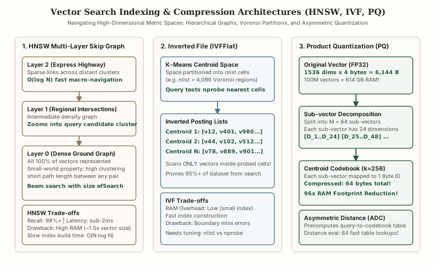
1. Layer 2 (Express Highway) & Layer 1 (Regional Intersections)
Establishes the ingress and structural boundary across Layer 2 (Express Highway) & Layer 1 (Regional Intersections): Sparse links across distant clusters O(log N) fast macro-navigation; Intermediate density graph Zooms into query candidate cluster; All 100% of vectors represented.
2. K-Means Centroid Space & Inverted Posting Lists
Coordinates core data-plane execution and state transitions through K-Means Centroid Space & Inverted Posting Lists: Space partitioned into nlist cells (e.g. nlist = 4,096 Voronoi regions) Query tests nprobe nearest cells; Centroid 1: [v12, v401, v980...]; Centroid 2: [v44, v102, v512...].
3. Original Vector (FP32) & Sub-vector Decomposition
Enforces durability, state convergence, and output verification across Original Vector (FP32) & Sub-vector Decomposition: 1536 dims x 4 bytes = 6,144 B 100M vectors = 614 GB RAM!; Split into M = 64 sub-vectors Each sub-vector has 24 dimensions; [D_1..D_24] [D_25..D_48] ...
The Small World Phenomenon
A Small World Graph is a network with two defining topological properties:
- High Clustering: Nodes that share a mutual neighbor are likely to be directly connected (dense local neighborhoods).
- Short Average Path Length: Any two arbitrary nodes in the entire graph can be reached in a small number of hops () via long-range “shortcuts”.
In a basic Navigable Small World (NSW) graph, searching is executed as a Greedy Routing algorithm: start at an entry node, evaluate distances to all neighbors, and hop to the neighbor closest to the query vector. Repeat until no neighbor is closer than the current node (local minimum).
However, basic NSW suffers from early stopping: greedy searches easily get trapped in local minima that are far from the true nearest neighbor.
The Hierarchical Skip-List Solution
HNSW solves local minima by generalizing the Skip-List to multi-dimensional graphs:
Layer 2 (Top Express Highway):
[ Node A ] ----------------------------------------------> [ Node K ]

Layer 1 (Regional Intersections):
[ Node A ] ----------> [ Node D ] ----------> [ Node G ] --> [ Node K ]

Layer 0 (Dense Ground Graph - All 100% Vectors):
[ Node A ] -> [ Node B ] -> [ Node C ] -> [ Node D ] -> [ Node E ] ... -> [ Node K ]- Layer Hierarchy:
- Every vector is assigned a maximum layer using an exponential probability distribution: .
- Layer 0 contains all vectors.
- Layer 1 contains roughly of the vectors.
- Layer 2 contains roughly of the vectors.
- Query Traversal Algorithm:
- Begin at the global entry node on the topmost layer ().
- Perform greedy search on to locate the local nearest neighbor.
- Using that local minimum as the entry point, descend to .
- Repeat greedy routing down through the layers. Upper layers act as high-speed express highways, executing macroscopic jumps across clusters in hops.
- Upon reaching Layer 0, switch from greedy 1-NN search to a Beam Search with priority queue size
efSearch(e.g., 64). The algorithm maintains the best candidates, exploring their local neighborhood to achieve recall.
Critical Tuning Parameters
- (e.g., 16–64): Maximum number of bidirectional connections per node. Higher improves recall on complex datasets but linearly increases RAM consumption.
efConstruction(e.g., 128–512): Size of the priority queue during index construction. Controls index build quality.efSearch(e.g., 32–256): Size of the priority queue during live queries. Allows run-time tuning: increaseefSearchfor high recall (), decrease for sub-millisecond latency.
4. Partition-Based Indexing: Inverted File Index (IVF)
While HNSW offers exceptional recall and speed, its graph edges consume significant memory (~20%–50% on top of raw vector storage). For massive datasets, Inverted File Indexing (IVF) offers a memory-efficient alternative.
The Voronoi Cell Architecture
IVF borrows the inverted index concept from search engines (like Lucene):
- Training Phase: The algorithm runs -means clustering across the vector dataset to establish
nlistcluster centroids (e.g., ). These centroids divide the high-dimensional space into Voronoi Cells. - Posting Lists: Each centroid maintains an inverted list of vector IDs assigned to its cell:
- Query Phase (
nprobe):- Given query , compute distance to all
nlistcentroids ( operations). - Select the
nprobeclosest centroids (e.g., ). - Scan only the vectors inside the posting lists of those 16 centroids, pruning of the dataset from evaluation!
- Given query , compute distance to all
+---------------------------------------------------------------------------------+
|                       The IVF Boundary Miss Hazard                              |
|                                                                                 |
| If a query vector lands near the boundary between two Voronoi cells, its true   |
| nearest neighbor might lie just across the border in an adjacent cell.          |
| If nprobe is set too low (e.g. nprobe = 1), the engine misses the true neighbor.|
| Solution: Tune nprobe dynamically to balance latency vs. recall.                |
+---------------------------------------------------------------------------------+
5. Vector Compression: Scalar & Product Quantization
A database with 100 million 1536-dimensional FP32 vectors consumes 614 GB of RAM just for raw floats. Vector Quantization compresses vector representations while preserving metric distances.
1. Scalar Quantization (SQ8)
Scalar Quantization maps continuous 32-bit floating point numbers () into 8-bit unsigned integers ():
- Compression Ratio: Exactly ( per dimension).
- 614 GB of RAM shrinks to 153.6 GB.
- Accuracy: Minimal recall loss (~1%–2%). Distance computations run on integer SIMD hardware instructions.
2. Product Quantization (PQ)
Product Quantization (Jegou et al., 2011) is the gold standard for radical memory reduction ( compression):
Original FP32 Vector (1536 dimensions = 6,144 bytes)
[ d_1 ... d_24 ] [ d_25 ... d_48 ] ... [ d_1513 ... d_1536 ]
       |                 |                      |
       v                 v                      v
  Sub-vector 1      Sub-vector 2          Sub-vector 64 (M = 64)
       |                 |                      |
   Quantize          Quantize               Quantize
       v                 v                      v
  Centroid #42      Centroid #18           Centroid #201 (k = 256 Centroids)
       |                 |                      |
  [ Byte 0x2A ]     [ Byte 0x12 ]          [ Byte 0xC9 ]
-----------------------------------------------------------------------------
Compressed Vector: Exactly 64 Bytes! (96x Memory Reduction)- Sub-vector Decomposition: Split vector of dimension into equal sub-vectors of dimension .
- Codebook Training: Run -means on each sub-space independently to produce centroids. Because , each centroid index fits into a single 8-bit byte ().
- Quantized Representation: Replace the original 6,144-byte vector with bytes representing the assigned centroid IDs.
Asymmetric Distance Computation (ADC)
How can you calculate the distance between an uncompressed query vector and a compressed 64-byte vector without decompressing all data?
The ADC Trick:
- Before scanning vectors, compute the distance between query sub-vector and all 256 centroids in codebook .
- Store the results in a small Query Distance Table of size floats (), which fits entirely into L1/L2 CPU Cache!
- To calculate the distance to any compressed vector, execute table lookups and sum the values:
Computing the distance between a 1536-dimensional query and a candidate vector requires 64 array lookups and additions—zero floating-point multiplications!
6. Hybrid Search & The Metadata Filtering Challenge
In enterprise RAG systems, queries are rarely pure vector searches. They almost always include relational filters:
SELECT document_id, vector_distance(embedding, :query_vec)
FROM enterprise_knowledge_base
WHERE organization_id = 'acme_corp'
  AND created_at >= '2026-01-01'
  AND classification = 'confidential'
ORDER BY vector_distance ASC
LIMIT 10;
Combining vector distance search with relational filtering introduces a fundamental architectural dilemma:
1. Pre-Filtering (Filter Vector Search)
- Mechanism: Execute SQL predicate first, collecting all matching IDs. Then, search for the nearest neighbor among those IDs.
- Failure Mode: Pre-filtering breaks HNSW graph navigation! If 90% of nodes in HNSW are filtered out, the graph becomes disconnected. Greedy search encounters dead ends where all neighbors of a node are disqualified, causing recall to collapse to near zero.
2. Post-Filtering (Vector Search Filter)
- Mechanism: Perform standard HNSW search to retrieve top (e.g., ) nearest vector neighbors. Discard any candidate that fails the metadata filter.
- Failure Mode: If the metadata filter is highly selective (e.g., matching only 0.01% of documents), none of the top 100 vectors will satisfy the filter. The database returns an empty result set even though matching documents exist!
3. Single-Stage Filtered HNSW (Iterative Graph Traversal)
Modern vector databases (e.g., Qdrant, Milvus) implement Single-Stage Filtered Navigation:
- Maintain metadata filters as bitsets or roaring bitmaps.
- During HNSW beam search, traversals can hop through disqualified nodes to reach other parts of the graph, but disqualified nodes are never admitted to the final result priority queue.
- If selectivity is extreme, the query planner automatically falls back to an exact inverted index scan.
7. Real-World Vector Database Comparison
| Architecture Dimension | Milvus | Qdrant | pgvector | Pinecone |
|---|---|---|---|---|
| Implementation Language | Go (Control) / C++ (Core) | Rust | C (Postgres Extension) | Proprietary / C++ |
| Primary Index Types | HNSW, IVF, DiskANN, SCaNN | HNSW with payload index | HNSW, IVFFlat | Proprietary Graph / IVF |
| Storage Architecture | Disaggregated (MinIO + Pulsar) | Embedded local NVMe storage | Co-located in PostgreSQL heap | Serverless Cloud-Native |
| Filtering Strategy | Plan-based single-stage bitsets | In-graph payload-aware traversal | Recheck filter or filtered index | Native hybrid planner |
| Best Suited For | Billion-scale distributed clusters | Millisecond RAG, high-concurrency | Existing Postgres stacks (<10M) | Fully managed SaaS |
8. Mathematical Capacity Planning: Memory Sizing
Memory Formula for HNSW Index
In canonical HNSW implementations (hnswlib, FAISS, Qdrant, Milvus), Layer 0 contains all vectors and allocates up to neighbor slots per node using 32-bit internal node IDs ( each, supporting up to vectors per segment on Layer 0, plus expected across upper layers ), alongside of external ID/level metadata and a operational memory buffer for active segment merges:
Sizing Scenario: Vectors (, )
- Raw Vector Memory:
- HNSW Graph Adjacency Overhead ( neighbor IDs ):
- Node ID & Layer Metadata ():
- Total with Operational Compaction Buffer:
Across a distributed cluster of 8 query nodes, each shard requires at least of DRAM to serve in-memory HNSW queries without swap thrashing.
If compressed with Product Quantization ( subspaces, ) inside an IVF-PQ index:
- Raw PQ Codes: ( raw vector compression vs. FP32).
- Full
IVF-PQIndex Footprint (adding vector IDs in posting lists , negligible centroid table, and operational headroom):
9. Concrete Implementation: In-Memory ANN Engine
The following complete TypeScript implementation demonstrates an Approximate Nearest Neighbor Engine featuring normalized vector math, a multi-layer HNSW Skip-Graph, and Product Quantization with Asymmetric Distance Computation:
export type Vector = Float32Array;

/**
 * High-performance vector math operations
 */
export class VectorOps {
  static dotProduct(a: Vector, b: Vector): number {
    let sum = 0;
    const len = a.length;
    for (let i = 0; i < len; i++) {
      sum += a[i] * b[i];
    }
    return sum;
  }

  static euclideanDistance(a: Vector, b: Vector): number {
    let sum = 0;
    const len = a.length;
    for (let i = 0; i < len; i++) {
      const diff = a[i] - b[i];
      sum += diff * diff;
    }
    return Math.sqrt(sum);
  }

  static normalize(v: Vector): Vector {
    let norm = 0;
    for (let i = 0; i < v.length; i++) norm += v[i] * v[i];
    norm = Math.sqrt(norm);
    if (norm === 0) return v;
    const res = new Float32Array(v.length);
    for (let i = 0; i < v.length; i++) res[i] = v[i] / norm;
    return res;
  }
}

export interface NodeRecord {
  id: string;
  vector: Vector;
  layer: number;
  metadata?: Record<string, string>;
}

/**
 * Hierarchical Navigable Small World (HNSW) Simplified Simulator
 */
export class HNSWIndex {
  private nodes = new Map<string, NodeRecord>();
  // adjacency[layer][nodeId] = Set<neighborNodeId>
  private adjacency: Map<string, Set<string>>[] = [];
  private entryPointId: string | null = null;
  private maxLayer = -1;
  private readonly M: number;
  private readonly efConstruction: number;
  private readonly mL: number;

  constructor(M = 16, efConstruction = 64) {
    this.M = M;
    this.efConstruction = efConstruction;
    this.mL = 1 / Math.log(M);
  }

  private sampleLayer(): number {
    return Math.floor(-Math.log(Math.random()) * this.mL);
  }

  insert(id: string, rawVector: Vector, metadata?: Record<string, string>): void {
    const vector = VectorOps.normalize(rawVector);
    const targetLayer = this.sampleLayer();
    const node: NodeRecord = { id, vector, layer: targetLayer, metadata };
    this.nodes.set(id, node);

    // Expand graph layers if necessary
    while (this.adjacency.length <= targetLayer) {
      this.adjacency.push(new Map());
    }

    if (this.entryPointId === null) {
      this.entryPointId = id;
      this.maxLayer = targetLayer;
      for (let l = 0; l <= targetLayer; l++) {
        this.adjacency[l].set(id, new Set());
      }
      return;
    }

    let currObj = this.nodes.get(this.entryPointId)!;
    let currDist = VectorOps.euclideanDistance(vector, currObj.vector);

    // 1. Top-down greedy search through layers above targetLayer
    for (let l = this.maxLayer; l > targetLayer; l--) {
      let changed = true;
      while (changed) {
        changed = false;
        const neighbors = this.adjacency[l].get(currObj.id) || new Set();
        for (const nId of neighbors) {
          const neighbor = this.nodes.get(nId)!;
          const d = VectorOps.euclideanDistance(vector, neighbor.vector);
          if (d < currDist) {
            currDist = d;
            currObj = neighbor;
            changed = true;
          }
        }
      }
    }

    // 2. Insert into targetLayer and below, connecting to M closest neighbors
    for (let l = Math.min(targetLayer, this.maxLayer); l >= 0; l--) {
      if (!this.adjacency[l].has(id)) this.adjacency[l].set(id, new Set());

      // Connect bidirectionally
      const neighbors = this.adjacency[l].get(id)!;
      neighbors.add(currObj.id);
      if (!this.adjacency[l].has(currObj.id)) this.adjacency[l].set(currObj.id, new Set());
      const currObjNeighbors = this.adjacency[l].get(currObj.id)!;
      currObjNeighbors.add(id);

      // Prune connections if exceeding M on both endpoints
      if (neighbors.size > this.M) {
        const sorted = Array.from(neighbors)
          .map((nId) => ({ id: nId, d: VectorOps.euclideanDistance(vector, this.nodes.get(nId)!.vector) }))
          .sort((a, b) => a.d - b.d);
        this.adjacency[l].set(id, new Set(sorted.slice(0, this.M).map((x) => x.id)));
      }
      if (currObjNeighbors.size > this.M) {
        const sortedPeer = Array.from(currObjNeighbors)
          .map((nId) => ({ id: nId, d: VectorOps.euclideanDistance(currObj.vector, this.nodes.get(nId)!.vector) }))
          .sort((a, b) => a.d - b.d);
        this.adjacency[l].set(currObj.id, new Set(sortedPeer.slice(0, this.M).map((x) => x.id)));
      }
    }

    if (targetLayer > this.maxLayer) {
      this.maxLayer = targetLayer;
      this.entryPointId = id;
    }
  }

  /**
   * Approximate Nearest Neighbor Search with efSearch beam search
   */
  search(queryVec: Vector, k: number, efSearch = 32): { id: string; distance: number; metadata?: Record<string, string> }[] {
    if (this.entryPointId === null) return [];
    const qNorm = VectorOps.normalize(queryVec);

    let currObj = this.nodes.get(this.entryPointId)!;
    let currDist = VectorOps.euclideanDistance(qNorm, currObj.vector);

    // 1. Greedy routing on express upper layers
    for (let l = this.maxLayer; l > 0; l--) {
      let changed = true;
      while (changed) {
        changed = false;
        const neighbors = this.adjacency[l].get(currObj.id) || new Set();
        for (const nId of neighbors) {
          const neighbor = this.nodes.get(nId)!;
          const d = VectorOps.euclideanDistance(qNorm, neighbor.vector);
          if (d < currDist) {
            currDist = d;
            currObj = neighbor;
            changed = true;
          }
        }
      }
    }

    // 2. Beam search on ground Layer 0
    const visited = new Set<string>([currObj.id]);
    const candidates = [{ id: currObj.id, dist: currDist }];
    const w = [{ id: currObj.id, dist: currDist }];

    while (candidates.length > 0) {
      candidates.sort((a, b) => a.dist - b.dist);
      const c = candidates.shift()!;

      w.sort((a, b) => a.dist - b.dist);
      const furthestResult = w[w.length - 1];

      if (c.dist > furthestResult.dist && w.length >= efSearch) {
        break; // Stop criteria
      }

      const neighbors = this.adjacency[0].get(c.id) || new Set();
      for (const nId of neighbors) {
        if (!visited.has(nId)) {
          visited.add(nId);
          const neighbor = this.nodes.get(nId)!;
          const d = VectorOps.euclideanDistance(qNorm, neighbor.vector);

          if (d < furthestResult.dist || w.length < efSearch) {
            candidates.push({ id: nId, dist: d });
            w.push({ id: nId, dist: d });
            if (w.length > efSearch) {
              w.sort((a, b) => a.dist - b.dist);
              w.pop(); // Evict furthest
            }
          }
        }
      }
    }

    w.sort((a, b) => a.dist - b.dist);
    return w.slice(0, k).map((item) => ({
      id: item.id,
      distance: item.dist,
      metadata: this.nodes.get(item.id)?.metadata,
    }));
  }
}

/**
 * Product Quantization (PQ) Codebook & Asymmetric Distance Computer (ADC)
 */
export class ProductQuantizer {
  public readonly D: number;
  public readonly M: number;
  public readonly subDim: number;
  public readonly kCentroids: number;
  // codebooks[subVectorIdx][centroidIdx] = Float32Array(subDim)
  private codebooks: Float32Array[][] = [];

  constructor(D = 128, M = 8, kCentroids = 256) {
    this.D = D;
    this.M = M;
    this.subDim = D / M;
    this.kCentroids = kCentroids;
    this.initSyntheticCodebooks();
  }

  private initSyntheticCodebooks(): void {
    // Generates initialized synthetic centroids for demonstration
    for (let m = 0; m < this.M; m++) {
      const centroids: Float32Array[] = [];
      for (let k = 0; k < this.kCentroids; k++) {
        const centroid = new Float32Array(this.subDim);
        for (let d = 0; d < this.subDim; d++) {
          centroid[d] = (Math.random() - 0.5) * 2;
        }
        centroids.push(centroid);
      }
      this.codebooks.push(centroids);
    }
  }

  encode(vector: Vector): Uint8Array {
    const codes = new Uint8Array(this.M);
    for (let m = 0; m < this.M; m++) {
      const subVec = vector.subarray(m * this.subDim, (m + 1) * this.subDim);
      let bestCentroid = 0;
      let minDist = Infinity;
      for (let k = 0; k < this.kCentroids; k++) {
        const dist = VectorOps.euclideanDistance(subVec, this.codebooks[m][k]);
        if (dist < minDist) {
          minDist = dist;
          bestCentroid = k;
        }
      }
      codes[m] = bestCentroid;
    }
    return codes;
  }

  computeDistanceTable(query: Vector): Float32Array[] {
    const table: Float32Array[] = [];
    for (let m = 0; m < this.M; m++) {
      const subQ = query.subarray(m * this.subDim, (m + 1) * this.subDim);
      const subDistances = new Float32Array(this.kCentroids);
      for (let k = 0; k < this.kCentroids; k++) {
        const diff = VectorOps.euclideanDistance(subQ, this.codebooks[m][k]);
        subDistances[k] = diff * diff;
      }
      table.push(subDistances);
    }
    return table;
  }

  asymmetricDistance(distanceTable: Float32Array[], encodedCodes: Uint8Array): number {
    let squaredDistance = 0;
    for (let m = 0; m < this.M; m++) {
      const centroidIdx = encodedCodes[m];
      squaredDistance += distanceTable[m][centroidIdx];
    }
    return Math.sqrt(squaredDistance);
  }
}

function runDemo(): void {
  console.log("=== Vector Search: HNSW & Product Quantization Demo ===");
  const index = new HNSWIndex(16, 64);
  const vectors: Record<string, Float32Array> = {
    "doc-1": new Float32Array([0.1, 0.9, 0.2, 0.1, 0.0, 0.4, 0.8, 0.3]),
    "doc-2": new Float32Array([0.8, 0.1, 0.9, 0.2, 0.7, 0.0, 0.1, 0.9]),
    "doc-3": new Float32Array([0.15, 0.85, 0.25, 0.1, 0.05, 0.35, 0.75, 0.28]),
  };
  for (const [id, vec] of Object.entries(vectors)) {
    index.insert(id, vec, { category: id === "doc-2" ? "storage" : "vector-ai" });
  }
  console.log(`Indexed 3 high-dimensional vectors into HNSW graph.`);
  const query = new Float32Array([0.12, 0.88, 0.22, 0.08, 0.02, 0.38, 0.78, 0.31]);
  const results = index.search(query, 2);
  console.log(`Top-2 Nearest Neighbors for query vector:`);
  for (const r of results) {
    console.log(`  Match: [${r.id}] (distance: ${r.distance.toFixed(4)}, category: ${r.metadata?.category})`);
  }
}

runDemo();
10. Failure Modes, Tombstone Degradation & Operational Recovery
| Failure Mode / Pitfall | Root Architectural Cause | Production Mitigation & Recovery |
|---|---|---|
| HNSW Tombstone Recall Degradation | Deleting a bridge node directly from HNSW severs multi-hop skip-list routing paths; engines instead mark deleted IDs in a soft-delete tombstone bitset. Above ~20% tombstones, beam search wastes efSearch budget visiting dead nodes. | Partition collections into immutable sealed segments (LSM-style, as in Qdrant/Milvus) and run background segment compaction to rebuild clean HNSW graphs and reclaim RAM. |
| Compaction Double-RAM Out-of-Memory (OOM) | Rebuilding a 64 GB HNSW segment in-place requires holding both the live serving graph and the newly constructed graph in DRAM simultaneously. | Reserve a strict DRAM headroom per query node, cap segment size (e.g., 512 MB–1 GB per segment), or offload index builds to dedicated asynchronous IndexNode workers. |
| IVF Voronoi Centroid Drift | An IVF/PQ codebook trained on 2024 product data becomes skewed as new out-of-distribution topics arrive, creating “hot” posting lists larger than average that spike p99 tail latency. | Monitor per-centroid posting-list variance (Gini/skew coefficient); trigger shadow re-clustering and dual-read index swap when max-to-median cell ratio exceeds . |
| Embedding Model Version Mixing | Upgrading from one embedding model to another (or changing normalization) rotates the latent vector manifold, causing cosine comparisons across versions to return random noise. | Enforce embedding_model_id schema constraints per collection and execute blue/green shadow backfills during model migrations. |
11. Summary & Decision Guide
+-----------------------------------------------------------------------------------+
|                        Vector Index Selection Matrix                              |
+---------------------+-------------------+-------------------+---------------------+
| Index Type          | Latency (QPS)     | Recall@10         | Memory Footprint    |
+---------------------+-------------------+-------------------+---------------------+
| Flat (Brute Force)  | Terrible (O(N*d)) | 100% (Exact)      | 1.00x (Raw Vectors) |
| HNSW (In-Memory)    | Blazing (1-3 ms)  | Superior (98%+)   | 1.05x - 1.35x (High)|
| HNSW + SQ8          | Blazing (1-3 ms)  | High (97%-99%)    | 0.28x - 0.35x (Med) |
| IVF-Flat            | Moderate (5-15 ms)| High (90%-95%)    | 1.02x (Baseline)    |
| IVF-PQ (Quantized)  | Fast (2-8 ms)     | Moderate (85%-92%)| 0.01x - 0.05x (Tiny)|
| DiskANN (Vamana)    | Fast (3-10 ms)    | High (95%+)       | NVMe SSD + PQ in RAM|
+---------------------+-------------------+-------------------+---------------------+
The AI Systems Architect’s Rule of Thumb
- Always Unit-Normalize: Pre-normalizing embedding vectors () converts expensive Cosine Similarities into hardware-accelerated SIMD Dot Products.
- Under 50M Vectors with Strict Recall Requirements: Select HNSW with SQ8 compression (plus FP32 oversampling rescore from NVMe). It delivers sub-3ms latency with Recall@10 at total RAM savings.
- Over 100M Vectors on Tight DRAM Budgets: Select IVF-PQ (with OPQ rotation and refine rescore) or DiskANN (Vamana). Keep compressed PQ codes in DRAM and fetch full vectors only for the top- rescore candidates.
- Never Rely on Blind Post-Filtering: When pairing vector search with selective metadata predicates, enforce single-stage filtered HNSW traversal backed by Roaring Bitmaps.
12. Guided Design Exercises
Exercise 1 (Foundational — HNSW vs. IVF-PQ Memory & ADC Cache Sizing)
You are architecting a vector search cluster for embeddings of dimension (FP32) with HNSW degree .
- Calculate the total DRAM required for an uncompressed in-memory HNSW index (including Layer-0 neighbor pointers, metadata per vector, and a compaction buffer).
- Calculate the compressed RAM footprint using
IVF-PQwith subspaces, centroids per subspace, and vector IDs (with operational buffer), and verify that the per-query Asymmetric Distance Computation (ADC) lookup table fits inside a CPU L1/L2 cache.
Exercise 2 (Intermediate — Single-Stage Filtered HNSW vs. Post-Filtering Recall)
A multi-tenant RAG index stores document chunks across enterprise customers. Tenant acme_corp owns chunks (selectivity ).
- Under naive Post-Filtering (fetching global top- nearest vectors first, then filtering by
tenant_id = 'acme_corp'), calculate the expected number of survivingacme_corpchunks and the probability that the query returns an empty result set. - Design a cost-based hybrid query planner that switches dynamically between an exact Roaring Bitmap SIMD scan and Single-Stage Filtered HNSW traversal based on filter selectivity and
efSearch.
Exercise 3 (Staff-Level — Tombstone Degradation & Zero-Downtime Segment Compaction)
A high-churn e-commerce catalog vector index receives . Soft-delete tombstones in an active HNSW segment exceed of nodes, degrading p99 query latency from to , while triggering an in-place HNSW rebuild causes an Out-Of-Memory (OOM) crash on the query node. Formulate the diagnostic telemetry checks, immediate mitigation, and LSM-style immutable segment architecture to bound both p99 latency and peak DRAM usage.
View Reference Architecture & Worked Solutions (AI-C04-001)
1. Worked Solution — Exercise 1: HNSW vs. IVF-PQ Memory & ADC Cache Sizing
- Uncompressed HNSW Memory ():
- Raw FP32 Vectors: ()
- Layer-0 Adjacency Pointers ( edges ):
- Node ID & Level Metadata ():
- Total with Compaction Buffer:
- Compressed
IVF-PQMemory () & ADC Table Size:- PQ Codes (): ( raw vector reduction)
- Posting List Vector IDs ():
- Codebook Centroids (): (negligible)
- Total
IVF-PQRAM with Headroom: - ADC Lookup Table Footprint: This fits directly inside a modern core’s L1/L2 cache, replacing FP32 multiply-adds per candidate with L1-resident table lookups.
2. Worked Solution — Exercise 2: Single-Stage Filtered HNSW & Cost-Based Query Planner
- Post-Filtering Recall Collapse Math ():
- Expected surviving candidates: .
- Probability of returning zero results despite valid
acme_corpchunks existing:
- Cost-Based Hybrid Filtered ANN Planner (Qdrant / Milvus Strategy):
- Maintain a per-tenant Roaring Bitmap inverted index over internal
uint32vector IDs. - Compute bitmap cardinality and selectivity before touching the HNSW graph:
- Low-Cardinality Regime ( or ): Bypass HNSW entirely! Iterate directly over the matching vector IDs in the Roaring Bitmap using AVX-512 SIMD dot products ( with exact recall).
- Moderate/High-Cardinality Regime (): Execute Single-Stage Filtered HNSW Traversal where beam search traverses all graph edges (using non-matching nodes as routing bridges) but only pushes nodes with
bitmap.contains(nodeId) == trueinto the top-efSearchresult queue.
- Maintain a per-tenant Roaring Bitmap inverted index over internal
3. Worked Solution — Exercise 3: Tombstone Compaction & Immutable Segment Architecture
- Diagnostic Telemetry: Monitor
segment_tombstone_ratio = deleted_vectors / total_vectors(alert at ) andhnsw_visited_nodes_per_query(which inflates by under tombstone ratio , as beam search wastes hops evaluating dead nodes). - Root Cause of OOM: Rebuilding a single monolithic mutable HNSW graph in-place requires allocating a second graph concurrently in DRAM ().
- Permanent Architectural Fix (LSM-Style Sealed Segments):
- Cap Maximum Segment Size: Partition each shard into smaller immutable sealed segments of ( vectors each), plus a small active append-only write segment.
- Bounded Compaction Memory: Compacting two segments requires only of transient DRAM (well within the headroom buffer), completely eliminating compaction OOMs.
- Disaggregated Index Workers: Offload heavy HNSW graph construction (
efConstruction = 200) to dedicated CPU/GPU IndexNodes (Milvus Knowhere pattern) that write completed segment files to object storage, allowing QueryNodes to mmap clean segments with zero CPU or memory spike on the live read path.
13. Authoritative References & Version Context
- Version Baseline: Architectural details and memory equations verified against Qdrant v1.11+, Milvus v2.4+ (Knowhere C++ engine), Meta FAISS v1.8+,
hnswlibv0.8+, and pgvector v0.7+. - Malkov & Yashunin (IEEE TPAMI 2018) — Efficient and Robust Approximate Nearest Neighbor Search Using Hierarchical Navigable Small World Graphs: Primary specification of HNSW probabilistic skip-graph layers, , and
efConstruction/efSearchbeam routing. - Jégou, Douze & Schmid (IEEE TPAMI 2011) — Product Quantization for Nearest Neighbor Search: Introduces subspace codebook quantization and Asymmetric Distance Computation (ADC) lookup tables.
- Johnson, Douze & Jégou (IEEE Trans. Big Data 2019) — Billion-Scale Similarity Search with GPUs (FAISS): Production
IVF-PQVoronoi partitioning, multi-probe selection, and SIMD/GPU distance kernels. - Subramanya et al. (NeurIPS 2019) — DiskANN: Fast Accurate Billion-point Nearest Neighbor Search on a Single Node: Vamana single-layer SSD-resident graph combined with in-RAM PQ coordinates.