Back-of-the-Envelope Estimation

1. The problem

Suppose a product team announces a new photo-sharing feature for $10\text{ million}$ daily active users. Without running a single calculation, an architecture review quickly spirals into speculation: one engineer insists on sharding metadata across twelve Cassandra nodes on day one, while another assumes a single 10 Gbps origin server can stream every photo directly without a Content Delivery Network (CDN).

Both instincts fail in opposite directions:

• Over-engineering metadata: As we will prove in five lines of arithmetic, five years of photo metadata fits comfortably under $1\text{ TB}$—well within a single primary PostgreSQL instance with read replicas. Prematurely sharding sacrifices ACID joins and adds months of operational complexity for zero gain.
• Under-provisioning bandwidth: Streaming $200\text{ million}$ daily $2\text{ MB}$ photo views drives $37\text{ Gbps}$ average ($74\text{ Gbps}$ peak) of egress traffic, instantly saturating a single $10\text{ Gbps}$ NIC if no CDN offloads edge reads.

SYSTEM ARCHITECTURE BLUEPRINTDISTRIBUTED SYSTEMS

⤢Expand

ARCHITECTURAL FLOW · STEP 1 OF 3

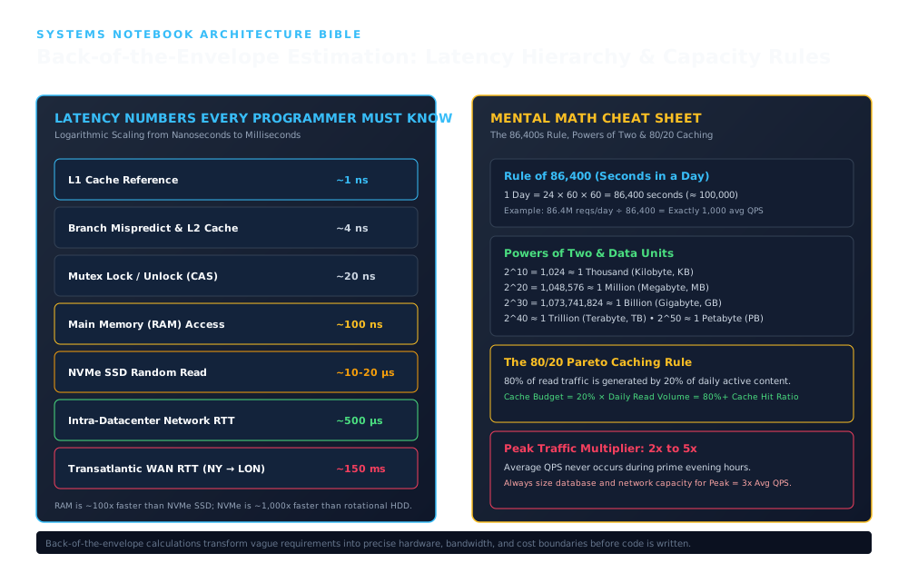
1. L1 Cache Reference & Branch Mispredict & L2 Cache

Establishes the ingress and structural boundary across L1 Cache Reference & Branch Mispredict & L2 Cache: ~20 ns; ~100 ns.

Architectural Invariant: Maintains deterministic distributed systems invariants across L1 Cache Reference & Branch Mispredict & L2 Cache.

ARCHITECTURAL FLOW · STEP 2 OF 3

2. NVMe SSD Random Read & Intra-Datacenter Network RTT

Coordinates core data-plane execution and state transitions through NVMe SSD Random Read & Intra-Datacenter Network RTT: ~10-20 μs; ~500 μs; ~150 ms.

Architectural Invariant: Example: 86.4M reqs/day ÷ 86,400 = Exactly 1,000 avg QPS.

ARCHITECTURAL FLOW · STEP 3 OF 3

3. Powers of Two & Data Units & The 80/20 Pareto Caching Rule

Enforces durability, state convergence, and output verification across Powers of Two & Data Units & The 80/20 Pareto Caching Rule: 2^10 = 1,024 ≈ 1 Thousand (Kilobyte, KB) 2^20 = 1,048,576 ≈ 1 Million (Megabyte, MB) 2^30 = 1,073,741,824 ≈ 1 Billion (Gigabyte, GB) 2^40 ≈ 1 Trillion (Terabyte, TB) • 2^50 ≈ 1 Petabyte (PB); 80% of read traffic is generated by 20% of daily active content. Cache Budget = 20% × Daily Read Volume = 80%+ Cache Hit Ratio; Average QPS never occurs during prime evening hours. Always size database and network capacity for Peak = 3x Avg QPS.

Architectural Invariant: 80% of read traffic is generated by 20% of daily active content. Cache Budget = 20% × Daily Read Volume = 80%+ Cache Hit Ratio.

Back-of-the-envelope estimation (“napkin math”) is the discipline of computing rapid order-of-magnitude bounds ($2\times \text{–}10\times$ precision) on QPS, storage, RAM working sets, and network bandwidth to validate physical feasibility before writing code.

2. Mental model

Treat capacity planning like municipal hydraulic engineering:

• Total volume = Durable storage capacity ($\text{GB},\text{TB},\text{PB}$ on SSD or object storage).
• Flow rate = Request throughput ($\text{QPS}$ / $\text{TPS}$) and byte throughput ($\text{MB/s}$).
• Pipe diameter = Network link capacity ($\text{Gbps}$, measured in bits per second, where $1\text{ Byte}=8\text{ bits}$) and PCIe/memory bus bandwidth.
• Pressurized local reservoir = In-memory caches ($\text{DRAM}$) absorbing repetitive read bursts so the deeper well (NVMe disk or database engine) does not saturate.

Whenever incoming peak flow exceeds the narrowest pipe or worker pool along the request path, queues grow nonlinearly until timeouts and dropped connections cascade upstream.

3. Core concepts & unit discipline

Decimal (SI) vs. Binary (IEC) Prefixes

Production capacity errors frequently stem from mixing decimal SI prefixes (used by network NICs, S3 billing, and SSD manufacturers) with binary powers of two (used by OS memory allocators and GiB VM RAM specs):

Seconds in a Day & Peak Traffic Multipliers

Real user traffic follows diurnal waves and event-driven spikes, so $k_{\text{peak}}$ typically ranges from $2\times$ to $5\times$ for consumer apps (and $10\times +$ for ticketing or flash-sale checkouts). For $10\text{ million}$ requests/day:

• $\text{Average QPS}=\frac{10,000,000}{86,400}\approx 116\text{ req/s}$ (mental shortcut: $\frac{10^7}{10^5}=100\text{ req/s}$).
• $\text{Peak QPS (at }3\times \text{)}\approx 348\text{ req/s}$.

4. Internal workings: The hardware latency hierarchy

Software architecture is governed by hardware physics. The table below reflects modern 2025–2026 server hardware (3–4 GHz Xeon/EPYC cores, DDR5 DRAM, PCIe 4.0/5.0 NVMe TLC SSDs) alongside a humanized time scale where $1\text{ ns}=1\text{ second}$:

Key architectural consequences:

1. DRAM vs. Flash Gap: Reading DRAM ($\sim 100\text{ ns}$) is $200\times$ to $700\times$ faster than an uncached NVMe flash read ($20\text{–}70\mu \text{s}$) and roughly $100,000\times$ faster than a rotational disk seek.
2. Network Serialization Tax: Replacing 20 in-process function calls with 20 sequential cross-service RPCs inside a datacenter ($20\times 500\mu \text{s}=10\text{ ms}$) burns the latency equivalent of $100,000$ DRAM accesses before executing any business logic.

5. Mathematics and worked example: Photo-sharing platform

Let us size a consumer photo-sharing platform end to end, stating every unit and assumption explicitly.

Workload Assumptions:

• Daily Active Users (DAU): $10\text{ Million}$ ($10^7$).
• Read Activity: Each active user views $20$ photos/day ($2\times 10^8$ views/day), diurnal peak factor $k_{\text{read}}=2\times$.
• Write Activity: $10\%$ of DAU upload $1$ photo/day ($10^6$ new photos/day), burst peak factor $k_{\text{write}}=3\times$.
• Payloads (Decimal SI): Average compressed photo blob $=2\text{ MB}$ ($2\times 10^6\text{ B}$); relational metadata row $=500\text{ B}$ (photo ID, user ID, creation timestamp, caption, object key).

Step 1: Throughput Estimation (QPS)

Conclusion: Read-to-write ratio is $200:1$. Writes are tiny ($35\text{ QPS}$ peak), whereas read delivery dominates capacity design.

Step 2: 5-Year Durable Storage Sizing

Binary Media (Object Storage):

$$\text{Daily Raw Media}=10^6\times 2\text{ MB}=2\text{ TB/day}$$ $$\text{5-Year Media}=2\text{ TB/day}\times 365\times 5=3,650\text{ TB}=3.65\text{ PB}(\approx 3.24\text{ PiB})$$

Relational Metadata (Database):

$$\text{Daily Raw Metadata}=10^6\times 500\text{ B}=500\text{ MB/day}=0.5\text{ GB/day}$$ $$\text{5-Year Raw Metadata}=0.5\text{ GB/day}\times 365\times 5=912.5\text{ GB}(\approx 850\text{ GiB})$$

Applying a $1.6\times$ B-tree index, tuple-header, and WAL overhead factor yields $912.5\text{ GB}\times 1.6=1.46\text{ TB}$ per database replica.

Conclusion: Media ($3.65\text{ PB}$) belongs in erasure-coded object storage (e.g., Amazon S3) with lifecycle tiering after 90 days. Metadata ($1.46\text{ TB}$ physical footprint over 5 years) fits easily on a single unsharded PostgreSQL primary + standby/read replicas.

Step 3: Network Bandwidth (Average and Peak, in Bits/Sec)

Always size NICs and CDN contracts for peak flow and multiply bytes by $8$:

Conclusion: Peak egress ($74.1\text{ Gbps}$) exceeds commodity single-VM NIC allocations. Offloading $\ge 92\%$ of image reads to an edge CDN (e.g., Cloudflare CDN / CloudFront) drops origin egress below $6\text{ Gbps}$.

Step 4: Cache Memory Sizing (80/20 Pareto Working Set)

Suppose feed ranking draws primarily from the active 200-million-photo catalog (~6.6 months of recent uploads, or equivalently upper-bounding distinct photos accessed on a busy day by $200\text{M}$). Under the 80/20 Pareto heuristic, caching the hottest $20\%$ of that active catalog serves $\sim 80\%$ of requests:

• Why not cache media blobs in server DRAM? $20\%\times 200\text{M}\times 2\text{ MB}=80\text{ TB}$ of DRAM—economically absurd when edge CDN SSD caches solve this cheaply.
• Cache metadata rows in Redis: $$\text{Active Candidate Metadata}=200\times 10^6\times 500\text{ B}=100\text{ GB}(\approx 93.1\text{ GiB})$$ $$\text{Hot 20\% Payload}=100\text{ GB}\times 0.20=20\text{ GB}(\approx 18.6\text{ GiB})$$ Accounting for $\sim 1.4\times$ Redis key-pointer, hash-bucket, and jemalloc overhead ($20\text{ GB}\times 1.4=28\text{ GB}\approx 26.1\text{ GiB}$), a single 32 GiB primary + replica Redis pair holds the entire hot metadata working set in memory.

6. Implementation: Capacity & Hardware Sizing Calculator in TypeScript

The calculator below distinguishes raw vs. physical storage overhead, converts peak byte rates into decimal $\text{Mbps}$, and computes binary $\text{GiB}$ Redis memory including allocator overhead.

export interface WorkloadProfile {
  dailyActiveUsers: number;
  writesPerUserPerDay: number;
  readsPerUserPerDay: number;
  writePayloadBytes: number;
  readMetadataBytes: number;
  activeCatalogItems: number;
  peakWriteMultiplier?: number;    // default 3.0
  peakReadMultiplier?: number;     // default 2.0
  replicationFactor?: number;      // default 3
  indexOverheadFactor?: number;    // default 1.5
  paretoWorkingSetRatio?: number;  // default 0.20
  cacheAllocatorOverhead?: number; // default 1.40 (Redis dict + jemalloc)
}

export interface CapacitySizingResult {
  writeQpsAvg: number;
  writeQpsPeak: number;
  readQpsAvg: number;
  readQpsPeak: number;
  dailyRawStorageTB: number;
  yearlyClusterStorageTB: number;
  peakIngressMbps: number;
  peakMetadataEgressMbps: number;
  recommendedCacheRamGiB: number;
}

export class CapacityEstimationCalculator {
  private static readonly SECONDS_PER_DAY = 86_400;
  private static readonly BYTES_PER_DECIMAL_TB = 1_000_000_000_000; // 10^12 B
  private static readonly BYTES_PER_BINARY_GIB = 1024 ** 3;         // 2^30 B

  public static calculate(profile: WorkloadProfile): CapacitySizingResult {
    const peakWrite = profile.peakWriteMultiplier ?? 3.0;
    const peakRead = profile.peakReadMultiplier ?? 2.0;
    const replication = profile.replicationFactor ?? 3;
    const indexOverhead = profile.indexOverheadFactor ?? 1.5;
    const pareto = profile.paretoWorkingSetRatio ?? 0.20;
    const cacheOverhead = profile.cacheAllocatorOverhead ?? 1.40;

    const totalWritesDay = profile.dailyActiveUsers * profile.writesPerUserPerDay;
    const totalReadsDay = profile.dailyActiveUsers * profile.readsPerUserPerDay;

    const writeQpsAvgExact = totalWritesDay / this.SECONDS_PER_DAY;
    const readQpsAvgExact = totalReadsDay / this.SECONDS_PER_DAY;

    const writeQpsAvg = Math.round(writeQpsAvgExact * 10) / 10;
    const writeQpsPeak = Math.round(writeQpsAvgExact * peakWrite);
    const readQpsAvg = Math.round(readQpsAvgExact);
    const readQpsPeak = Math.round(readQpsAvgExact * peakRead);

    const dailyRawBytes = totalWritesDay * profile.writePayloadBytes;
    const dailyRawStorageTB =
      Math.round((dailyRawBytes / this.BYTES_PER_DECIMAL_TB) * 100) / 100;

    const yearlyClusterBytes = dailyRawBytes * 365 * replication * indexOverhead;
    const yearlyClusterStorageTB =
      Math.round((yearlyClusterBytes / this.BYTES_PER_DECIMAL_TB) * 100) / 100;

    // Network bandwidth uses decimal SI bits/sec (1 Mbps = 10^6 bits/sec)
    const peakIngressMbps =
      Math.round(((writeQpsPeak * profile.writePayloadBytes * 8) / 1_000_000) * 10) / 10;
    const peakMetadataEgressMbps =
      Math.round(((readQpsPeak * profile.readMetadataBytes * 8) / 1_000_000) * 10) / 10;

    // Cache working set: 20% of distinct active catalog * payload * allocator factor, in binary GiB
    const hotPayloadBytes =
      profile.activeCatalogItems * pareto * profile.readMetadataBytes * cacheOverhead;
    const recommendedCacheRamGiB =
      Math.round((hotPayloadBytes / this.BYTES_PER_BINARY_GIB) * 10) / 10;

    return {
      writeQpsAvg,
      writeQpsPeak,
      readQpsAvg,
      readQpsPeak,
      dailyRawStorageTB,
      yearlyClusterStorageTB,
      peakIngressMbps,
      peakMetadataEgressMbps,
      recommendedCacheRamGiB,
    };
  }
}

export function runDemo(): void {
  console.log('=== Capacity Estimation: Photo-Sharing Platform Sizing ===');
  const profile: WorkloadProfile = {
    dailyActiveUsers: 10_000_000,
    writesPerUserPerDay: 0.1,        // 1M photo uploads/day
    readsPerUserPerDay: 20,          // 200M photo views/day
    writePayloadBytes: 2_000_000,    // 2 MB (decimal SI) compressed image
    readMetadataBytes: 500,          // 500 B metadata record
    activeCatalogItems: 200_000_000, // 200M active candidate photos
    peakWriteMultiplier: 3.0,
    peakReadMultiplier: 2.0,
    replicationFactor: 3,            // 3x object-store / replica durability
    indexOverheadFactor: 1.0,        // raw object blobs (no B-tree index on blobs)
    paretoWorkingSetRatio: 0.20,
    cacheAllocatorOverhead: 1.40,
  };

  const sizing = CapacityEstimationCalculator.calculate(profile);

  console.log(`[Throughput] Write QPS: ${sizing.writeQpsAvg} avg (${sizing.writeQpsPeak} peak)`);
  console.log(`[Throughput] Read QPS: ${sizing.readQpsAvg} avg (${sizing.readQpsPeak} peak)`);
  console.log(`[Storage] Daily Raw Media Upload: ${sizing.dailyRawStorageTB} TB`);
  console.log(`[Storage] 1-Year Replicated Media Footprint (3x): ${sizing.yearlyClusterStorageTB} TB`);
  console.log(
    `[Network] Peak Media Ingress: ${sizing.peakIngressMbps} Mbps | Peak Metadata API Egress: ${sizing.peakMetadataEgressMbps} Mbps`
  );
  console.log(
    `[Caching] Hot Metadata Redis Footprint (20% Pareto + 1.4x Allocator): ${sizing.recommendedCacheRamGiB} GiB`
  );
}

runDemo();

Simulation Execution Output & State Transitions

=== Capacity Estimation: Photo-Sharing Platform Sizing ===
[Throughput] Write QPS: 11.6 avg (35 peak)
[Throughput] Read QPS: 2315 avg (4630 peak)
[Storage] Daily Raw Media Upload: 2 TB
[Storage] 1-Year Replicated Media Footprint (3x): 2190 TB
[Network] Peak Media Ingress: 560 Mbps | Peak Metadata API Egress: 18.5 Mbps
[Caching] Hot Metadata Redis Footprint (20% Pareto + 1.4x Allocator): 26.1 GiB

7. Design alternatives & capacity trade-offs

Capacity estimates directly dictate which architectural alternative is physically and economically viable:

8. Real-world implementation

1. Discord (Gateway Connection Memory Sizing): By measuring per-WebSocket Erlang/Elixir process and buffer overhead ($\sim 10\text{–}15\text{ KiB}$ per idle session), Discord capacity-plans gateway nodes for hundreds of thousands of concurrent connections while leaving headroom for burst fan-out serialization.
2. X / Twitter (Home Timeline RAM Budgeting): Caching materialized home timelines stores compact 64-bit tweet/user identifiers ($\sim 800\text{ entries}\times 16\text{–}24\text{ B}$ including structure metadata $\approx 15\text{–}20\text{ KiB}$ per active user) in Redis clusters rather than full tweet JSON payloads, shrinking cluster RAM by an order of magnitude.
3. Netflix Open Connect (Edge Bandwidth & Pareto Caching): Netflix embeds custom storage appliances ($100\text{–}400\text{ Gbps}$ NICs backed by NVMe flash) directly inside ISP peering facilities; overnight off-peak fills pre-populate the regional Pareto working set of titles so $>95\%$ of evening peak video traffic never traverses backbone transit.

9. Failure modes and limitations

1. The Average Fallacy: Provisioning for daily average QPS rather than peak QPS. Queueing delay explodes asymptotically as utilization $\rho =\lambda /\mu \to 1$ during the peak hour, causing timeouts even when 24-hour average CPU looks like $25\%$.
2. Bytes-vs.-Bits ($8\times$) & SI-vs.-IEC ($10\%$) Confusion: Calculating $1\text{ GB/s}$ of payload transfer and provisioning a $1\text{ Gbps}$ NIC ($125\text{ MB/s}$ actual ceiling) saturates the network link at $12.5\%$ of expected load.
3. Cloud Instance Network & EBS IOPS Ceilings: Sizing vCPUs and disk capacity while ignoring per-instance AWS EBS bandwidth caps or burstable NIC credit depletion.
4. Ignoring Storage & Memory Amplification: Provisioning exact raw byte volume without multiplying by $1.5\times \text{–}2.0\times$ for B-tree indexes, WAL segments, LSM compaction headroom, or Redis key/allocator fragmentation.

10. Operational perspective

Estimation Validation Loop

[Napkin Estimate] ──► [Baseline Prototype] ──► [Open-Loop Load Test] ──► [Production Telemetry]
        ▲                                                                          │
        └─────────────────────── Calibrate Unit Costs ($/QPS, ms/IO) ──────────────┘

• Unit-Cost Benchmarking: Treat napkin math as an initial hypothesis. Run an open-loop load generator (wrk2, k6) against a single node to measure empirical saturation QPS, bytes per record, and $p99$ latency before multiplying out cluster size.
• Utilization Headroom: Alert and autoscale at $65\%\text{–}70\%$ of measured CPU, NIC, or connection-pool saturation so traffic bursts and single-AZ failovers never push surviving nodes past the queueing knee.

11. Knowledge check

Review the interactive assessment quiz at the end of this lesson to verify your fluency with daily-to-QPS conversions, bytes-to-Gbps bandwidth math, DRAM-vs.-NVMe latency ratios, and Pareto cache sizing.

12. Exercises

Exercise 1: URL Shortener Capacity

• Requirements: $500\text{ Million}$ new URLs shortened per 30-day month. Read-to-write (redirect-to-create) ratio is $100:1$, with a $3\times$ peak multiplier. Records are retained for 5 years at $500\text{ bytes}$ raw payload per mapping ($1.6\times$ index/WAL overhead).
• Tasks:
  1. Compute average write QPS, average read QPS, and peak read QPS (using $30\times 86,400=2,592,000\text{ s/month}$).
  2. Calculate 5-year raw database storage and physical storage per replica including $1.6\times$ index overhead.
  3. Calculate peak HTTP redirect egress bandwidth in $\text{Mbps}$ assuming an $800\text{-byte}$ HTTP 302 response header+body, and size a Redis cache for the hottest $20\%$ of the 5-year dataset (including $1.4\times$ allocator overhead).

13. Summary and decision guide

14. Authoritative References & Version Context

• Hardware Baseline Context: Latency figures in Section 4 reflect 2025–2026 server platforms: 4th/5th-Gen Intel Xeon Scalable and AMD EPYC 9004/9005 CPUs, DDR5-4800/5600 ECC DRAM ($\sim 80\text{–}100\text{ ns}$ random uncached access), and enterprise PCIe 4.0/5.0 NVMe 2.0 TLC SSDs (e.g., Micron 7450 / Samsung PM9A3, $\sim 20\text{–}70\mu \text{s}$ QD=1 4 KiB read).
• Jeff Dean, “Designs, Lessons and Advice from Building Large Distributed Systems”, Keynote at ACM SIGOPS LADIS Workshop / Stanford CS295 — origin of the canonical “Numbers Everyone Should Know” latency hierarchy and back-of-the-envelope design methodology.
• Colin Scott and Peter Norvig, “Latency Numbers Every Programmer Should Know (Historical & Modern Hardware Progression)” / Norvig’s Design Calculations — tracks hardware latency evolution across CPU caches, DRAM, flash media, and WAN fiber.
• Redis Official Documentation, “Memory Optimization and Key/Allocator Overhead” — details dictEntry, robj, SDS header, and jemalloc fragmentation multipliers required for accurate working-set RAM sizing.
• AWS Documentation, “Amazon EC2 Instance Network Bandwidth & EBS I/O Performance Specifications” — production reference for baseline vs. burst NIC Gbps and storage throughput limits on cloud VMs.