A pervasive design anti-pattern in distributed software engineering is jumping straight to multi-node distributed architectures—introducing network hops, distributed locking, Raft consensus clusters, and cross-shard transactions—without ever measuring what a single, well-architected machine can achieve.
A single modern dual-socket server can host CPU cores, of RAM, NICs, and enterprise NVMe drives sustaining IOPS. When written with mechanical sympathy (asynchronous I/O, cache line awareness, zero-copy serialization), a single server can comfortably process to requests per second.
This lesson establishes the quantitative engineering foundations of single-node capacity, the minimum bottleneck envelope, Little’s Law, and the saturation knee.
1. Problem and Motivation
Consider an engineering team tasked with building an authentication and user-profile service expected to handle queries per second (QPS). The team immediately designs an elaborate 15-node Kubernetes cluster with distributed caching and multi-master database replication.
Within three months:
- Microservice network hops add of serialization and round-trip delay.
- Intermittent network partitions trigger leader election flaps.
- Cloud hosting bills exceed $15,000/month.
Had the team conducted a first-principles capacity estimate, they would have discovered that a single server with an in-memory cache handles at a p99 latency for $120/month.
Before distributing, engineers must answer three questions:
- What is the theoretical physical capacity ceiling of a single node?
- Which hardware subsystem (CPU, memory, storage, NIC, OS sockets) will be the first bottleneck?
- At what offered load does the system cross its saturation knee, causing tail latency collapse?
2. Mental Model: The Hardware Bottleneck Envelope
A server is not an abstract compute cloud; it is a finite collection of interconnected hardware components governed by physics:
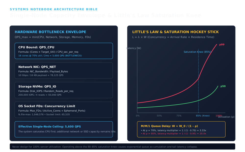
1. CPU Bound: QPS_CPU & Network NIC: QPS_NET
Establishes the ingress and structural boundary across CPU Bound: QPS_CPU & Network NIC: QPS_NET: Formula: (Cores × Target_Util) / CPU_sec_per_req; 16 cores @ 70% util / 2ms = 5,600 QPS (BOTTLENECK); Formula: NIC_Bandwidth / Payload_Bytes.
2. Storage NVMe: QPS_IO & OS Socket FDs: Concurrency Limit
Coordinates core data-plane execution and state transitions through Storage NVMe: QPS_IO & OS Socket FDs: Concurrency Limit: Formula: Disk_IOPS / Random_Reads_per_req; 200,000 IOPS / 4 reads = 50,000 QPS; Formula: Max_FDs / (Active_Conns + Ephemeral_Ports).
3. M/M/1 Queue Delay: W = W_0 / (1 - ρ) & Never design for 100% server utilization. Operating above the 80–85% saturation knee causes exponential queue accumulation and tail latency collapse.
Enforces durability, state convergence, and output verification across M/M/1 Queue Delay: W = W_0 / (1 - ρ) & Never design for 100% server utilization. Operating above the 80–85% saturation knee causes exponential queue accumulation and tail latency collapse.: At ρ = 70%, latency multiplier = 1 / (1 - 0.70) = 3.33x; At ρ = 95%, latency multiplier = 1 / (1 - 0.95) = 20.0x.
The overall maximum throughput is bounded by the weakest link in the hardware envelope:
If CPU allows but storage disk I/O caps out at , the server will saturate at , leaving of CPU capacity idle.
3. Core Formulas & Mathematical Derivations
3.1 The CPU Capacity Equation
For CPU-bound workloads (JSON serialization, cryptography, business logic), capacity is derived from available core seconds:
Where:
- is the number of physical or virtual CPU cores.
- is the target peak utilization ratio (, reserving headroom for spikes).
- is the average CPU compute time (in seconds) consumed per request (measured via profiling, e.g.
perfortime).
Example Calculation:
Assume a server with ( CPU utilization). Profiling reveals that parsing JSON and evaluating authorization takes .
3.2 Little’s Law and Steady-State Concurrency
Little’s Law is a fundamental theorem of queuing theory:
Where:
- is the average number of concurrent requests in the system (in-flight requests).
- is the average arrival rate (throughput in requests per second).
- is the average residence time (latency from arrival to response completion, in seconds).
Practical Implication: Worker Pool Sizing
If an API receives with an average downstream database latency of :
If the application runtime uses synchronous worker threads (e.g., Python WSGI or Ruby Unicorn), the server must allocate at least 150 worker threads and 150 database connection pool handles simply to avoid queuing incoming requests.
3.3 The Saturation Knee and the M/M/1 Queue Explosion
Why does latency explode when a server reaches CPU utilization?
In an idealized queue (Poisson arrivals, exponential service times), the average total response time is a function of service time and resource utilization :
Let us analyze the latency expansion factor :
| Utilization () | Latency Multiplier | Operational Assessment |
|---|---|---|
| () | Ample headroom, low queue delay | |
| () | Recommended production operating sweet spot | |
| () | The Saturation Knee: queue delay begins accelerating | |
| () | High tail-latency variance; minor bursts cause queue drops | |
| () | Severe degradation; p99 latency collapses | |
| () | Complete systemic brownout; timeouts and client retries |
4. Production TypeScript Simulation: Little’s Law & Saturation Engine
Here is a discrete-event simulator verifying Little’s Law and demonstrating how the saturation knee triggers exponential queue growth:
export interface RequestRecord {
  id: number;
  arrivalTimeMs: number;
  serviceTimeMs: number;
  startTimeMs: number;
  completionTimeMs: number;
}

export class SingleNodeQueueSimulator {
  private inFlight = 0;
  private queue: RequestRecord[] = [];
  private completed: RequestRecord[] = [];

  constructor(
    public readonly workerCapacity: number,
    public readonly baseServiceTimeMs: number
  ) {}

  public runSimulation(
    arrivalRatePerSec: number,
    durationSec: number
  ): {
    measuredQPS: number;
    averageConcurrencyL: number;
    expectedConcurrencyLittlesLaw: number;
    meanLatencyMs: number;
    p95LatencyMs: number;
    p99LatencyMs: number;
    utilizationPercent: number;
  } {
    const totalRequests = Math.floor(arrivalRatePerSec * durationSec);
    const timeline: { timeMs: number; type: "ARRIVE" | "FINISH"; req: RequestRecord }[] = [];

    // 1. Generate Poisson arrivals
    let currentTime = 0;
    for (let i = 0; i < totalRequests; i++) {
      // Exponential inter-arrival time: -ln(U) / lambda
      const interArrivalMs = (-Math.log(Math.random() || 1e-7) / arrivalRatePerSec) * 1000;
      currentTime += interArrivalMs;

      // Exponential service time
      const serviceTimeMs = (-Math.log(Math.random() || 1e-7) * this.baseServiceTimeMs);
      const req: RequestRecord = {
        id: i,
        arrivalTimeMs: currentTime,
        serviceTimeMs,
        startTimeMs: 0,
        completionTimeMs: 0,
      };
      timeline.push({ timeMs: currentTime, type: "ARRIVE", req });
    }

    // Sort timeline by event timestamp
    timeline.sort((a, b) => a.timeMs - b.timeMs);

    // 2. Discrete event simulation
    let simTime = 0;
    let activeWorkers = 0;
    const workerAvailableAt: number[] = new Array(this.workerCapacity).fill(0);
    const latencies: number[] = [];

    for (const event of timeline) {
      simTime = event.timeMs;

      // Find earliest available worker
      workerAvailableAt.sort((a, b) => a - b);
      const workerFreeTime = workerAvailableAt[0];

      const start = Math.max(simTime, workerFreeTime);
      const completion = start + event.req.serviceTimeMs;

      event.req.startTimeMs = start;
      event.req.completionTimeMs = completion;
      workerAvailableAt[0] = completion;

      const totalLatency = completion - event.req.arrivalTimeMs;
      latencies.push(totalLatency);
      this.completed.push(event.req);
    }

    latencies.sort((a, b) => a - b);
    const totalResidenceTimeSec = latencies.reduce((sum, v) => sum + v, 0) / 1000;
    const meanLatency = (totalResidenceTimeSec * 1000) / latencies.length;
    const p95 = latencies[Math.floor(latencies.length * 0.95)];
    const p99 = latencies[Math.floor(latencies.length * 0.99)];

    const arrivalWindowSec = simTime / 1000;
    const totalDurationSec = Math.max(simTime, Math.max(...workerAvailableAt)) / 1000;
    const measuredQPS = totalRequests / arrivalWindowSec;

    // Empirical time-average concurrency: integral of active requests over total simulation window
    const empiricalConcurrencyL = totalResidenceTimeSec / totalDurationSec;
    // Theoretical Little's Law concurrency: lambda * W
    const expectedConcurrencyLittlesLaw = measuredQPS * (meanLatency / 1000);

    // Concurrency sampled across timeline
    const utilization = (measuredQPS * (this.baseServiceTimeMs / 1000)) / this.workerCapacity;

    return {
      measuredQPS: Math.round(measuredQPS),
      averageConcurrencyL: parseFloat(empiricalConcurrencyL.toFixed(2)),
      expectedConcurrencyLittlesLaw: parseFloat(expectedConcurrencyLittlesLaw.toFixed(2)),
      meanLatencyMs: parseFloat(meanLatency.toFixed(2)),
      p95LatencyMs: parseFloat(p95.toFixed(2)),
      p99LatencyMs: parseFloat(p99.toFixed(2)),
      utilizationPercent: parseFloat((Math.min(utilization, 1.0) * 100).toFixed(1)),
    };
  }
}

function runDemo(): void {
  console.log("=== Little's Law & Single Node Queue Capacity Simulation ===");
  const sim = new SingleNodeQueueSimulator(16, 10);
  const result = sim.runSimulation(500, 1); // 500 req/sec over 1 sec
  console.log(`Arrival Rate: ${result.measuredQPS.toFixed(0)} QPS, Mean Latency: ${result.meanLatencyMs.toFixed(2)}ms`);
  console.log(`Average Concurrency L: ${result.averageConcurrencyL.toFixed(2)} concurrent requests`);
  console.log(`Expected Little's Law L: ${result.expectedConcurrencyLittlesLaw.toFixed(2)} (Utilization: ${result.utilizationPercent.toFixed(1)}%)`);
}

runDemo();
5. Real-World Production Architecture Analysis
A. Redis: Single-Threaded Core Scaling
Redis famously handles over on a single CPU core for simple commands (GET/SET).
- Why it scales: By executing on a single execution thread pinned to a core, Redis completely eliminates mutex lock contention, thread context-switching overhead, and false-sharing CPU cache invalidations.
- Where it hits the knee: Redis becomes CPU-bound when clients execute operations (
KEYS *,HGETALLon massive sets) or when JSON serialization consumes CPU time, stalling the event loop.
B. NGINX: Worker Process Core Affinity
NGINX configures worker_processes auto; and worker_cpu_affinity. By binding each single-threaded asynchronous worker process to a dedicated CPU core, NGINX maximizes L1/L2 cache locality and avoids CPU migration thrashing across NUMA nodes.
6. Failure Modes & Operational War Stories
War Story: The Ephemeral Socket Port Exhaustion Incident
- Symptoms: An API gateway began throwing intermittent
connect() failed (99: Cannot assign requested address)errors during a flash sale, despite CPU utilization being only . - Root Cause: The gateway made short-lived HTTP/1.0 downstream requests to microservices without connection pooling. The Linux kernel assigns ephemeral ports from
net.ipv4.ip_local_port_range( to ports). When TCP sockets close, they remain in theTIME_WAITstate for (2 * MSL). At , all ephemeral ports were exhausted in ! - Mitigation:
- Enabled HTTP/1.1 persistent connection pooling (
keepalive 256;). - Tuned kernel sysctl parameters:
net.ipv4.tcp_tw_reuse = 1and expanded port rangenet.ipv4.ip_local_port_range = 10240 65535.
- Enabled HTTP/1.1 persistent connection pooling (
7. Operational Decision Guide
| System Symptom | Identified Bottleneck | Required Remedy |
|---|---|---|
| CPU , run queue , p99 latency spikes | CPU Compute Bound | Optimize code/serialization, scale vertically (more cores), or add instances. |
CPU , disk iostat %util > 95%, high await | Storage I/O Bound | Add in-memory cache (Redis), migrate to PCIe NVMe, batch disk writes. |
Dropped SYN packets, high softirq (ksoftirqd), network latency | NIC PPS / Driver Bound | Enable Receive Side Scaling (RSS), jumbo frames, or kernel bypass (DPDK/XDP). |
Cannot assign requested address | Socket Port Exhaustion | Enable HTTP Keep-Alive connection pooling, enable tcp_tw_reuse. |
8. Hands-on Operational Drills
- Calculate Server Envelope: A server has vCPUs, NIC, and dual NVMe SSDs ( read IOPS). Each API request takes CPU time, generates response payload, and performs random NVMe reads. Calculate the limiting bottleneck QPS.
- Result: CPU is the strict bottleneck at .
- Run Queue Simulation: Execute
SingleNodeQueueSimulatorwith workers and base latency. Step through arrival rates from to and plot the hockey-stick p99 latency curve.
View Reference Architecture & Worked Solutions (CORE-M07A-001)
Drill 1: Complete Single-Node Bottleneck Envelope & Connection Pool Sizing
- Hardware Envelope Breakdown (, NIC, ):
- CPU Capacity Ceiling (, ):
- Network Egress Ceiling (, ):
- NVMe Storage Read Ceiling (, ):
- Minimum Bottleneck & Concurrency at Peak (): Assuming each NVMe read takes ( total I/O) plus CPU plus queueing delay (), Little’s Law yields:
Drill 2: Queueing Saturation Curve ( Workers, , )
export function plotSaturationCurve(): void {
  const rates = [100, 300, 500, 700, 800, 900, 950];
  for (const lambda of rates) {
    const sim = new SingleNodeQueueSimulator(10, 10); // Max service rate = 10 / 0.010s = 1000 QPS
    const res = sim.runSimulation(lambda, 5);
    console.log(
      `λ=${lambda} QPS (ρ=${res.utilizationPercent}%) | Mean=${res.meanLatencyMs}ms | p99=${res.p99LatencyMs}ms | L_emp=${res.averageConcurrencyL} vs L_Little=${res.expectedConcurrencyLittlesLaw}`
    );
  }
}- Empirical Hockey-Stick Progression:
- (): Zero queueing backlog; mean latency stays flat near and (pure exponential service-time tail).
- (, The Saturation Knee): Mean latency rises to , and crosses .
- (): Queueing delay dominates (), driving above and proving why production autoscalers must trigger at .
9. Design Alternatives & Capacity Trade-Off Matrix
| Concurrency Model | Target Utilization () | Latency Degradation Profile | Bottleneck Mechanism | Best Architectural Fit |
|---|---|---|---|---|
| Thread-per-Request (Tomcat / Django) | Severe hockey-stick latency spike above 80% | OS thread context switching and stack RAM | Enterprise CRUD systems, blocking JDBC drivers | |
| Event-Driven Non-Blocking (Node / Netty) | Predictable until event-loop lag increases | CPU-bound callbacks blocking event loop | I/O-intensive network proxies, WebSocket gateways | |
| Work-Stealing Task Pool (Tokio / Go) | Low latency variance across multi-core CPUs | Thread synchronization and work stealing overhead | High-performance microservices, API aggregators | |
| Stage Event-Driven SEDA (LMAX Disruptor) | Ultra-flat latency tail up to physical saturation | Ring buffer capacity and CPU core affinity | High-frequency trading, real-time telemetry matching |
10. Authoritative References & Version Context
- John D. C. Little (1961), “A Proof for the Queuing Formula: L = λ W”, Operations Research 9(3), pp. 383–387 — doi.org/10.1287/opre.9.3.383
- Leonard Kleinrock (1975), “Queueing Systems, Volume 1: Theory”, John Wiley & Sons: Comprehensive M/M/1 and M/G/1 queueing delay derivations — wiley.com
- Neil J. Gunther (2007), “Guerrilla Capacity Planning: A Tactical Approach to Practical System Performance”, Springer: Universal Scalability Law (USL) formulation — springer.com
- Version Context: Mathematical derivations are invariant over time; empirical benchmarking examples reflect Linux kernel 6.x CFS/EEVDF scheduler and modern 64-core x86-64 / ARMv9 architectures.